Download
1 / 27
270 likes | 501 Vues
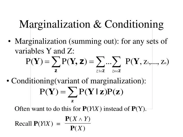
Marginalization & Conditioning. Marginalization (summing out): for any sets of variables Y and Z:. Conditioning(variant of marginalization):. Example of Marginalization. Using the full joint distribution. P(cavity) = P(cavity, toothache, catch) + P(cavity, toothache, catch) +

E N D
Marginalization & Conditioning • Marginalization (summing out): for any sets of variables Y and Z: • Conditioning(variant of marginalization):
Example of Marginalization • Using the full joint distribution P(cavity) = P(cavity, toothache, catch) + P(cavity, toothache, catch) + P(cavity, toothache, catch) + P(cavity, toothache, catch) = 0.108 +0.012 + 0.072 + 0.008 = 0.2
Inference By Enumeration using Full Joint Distribution • Let X be a random variable about which we want to know its probabilities, given some evidence (values e for a set E of other variables). Let the remaining (unobserved, so-called hidden) variables be Y. The query is P(X|e), and it can be answered using the full joint distribution by
Example of Inference By Enumeration using Full Joint Distribution
Independence • Propositions a and b are independent if and only if • Equivalently (by product rule): • Equivalently:
Illustration of Independence • We know (product rule) that
Illustration continued • Allows us to represent a 32-element table for full joint on Weather, Toothache, Catch, Cavity by an 8-element table for the joint of Toothache, Catch, Cavity, and a 4-element table for Weather. • If we add a Boolean variable X to the 8-element table, we get 16 elements. A new 2-element table suffices with independence.
Conditional Independence • X and Y are conditionally independentgivenZ if and only if P(X,Y|Z) = P(X|Z) P(Y|Z). • Y1,…,Ynare conditionally independent given X1,…,Xmif and only if P(Y1,…,Yn|X1,…,Xm)= P(Y1|X1,…,Xm) P(Y2|X1,…,Xm) … P(Ym|X1,…,Xm). • We’ve reduced 2n2m to 2n2m. Additional conditional independencies may reduce 2m.
Conditional Independence • As with absolute independence, the equivalent forms of X and Y being conditionally independent given Z can also be used: P(X|Y, Z) = P(X|Z) and P(Y|X, Z) = P(Y|Z)
Benefits of Conditional Independence • Allows probabilistic systems to scale up (tabular representations of full joint distributions quickly become too large.) • Conditional independence is much more commonly available than is absolute independence.
Decomposing a Full Joint by Conditional Independence • Might assume Toothache and Catch are conditionally independent given Cavity: P(Toothache,Catch|Cavity) = P(Toothache|Cavity) P(Catch|Cavity). • Then P(Toothache,Catch,Cavity) =[product rule]P(Toothache,Catch|Cavity) P(Cavity) =[conditional independence]P(Toothache|Cavity) P(Catch|Cavity) P(Cavity).
Naive Bayes Algorithm Let Fi be the i-th feature having valuej and Out be the target feature. • We can use training data to estimate: P(Fi = vj) P(Fi = vj | Out = True) P(Fi = vj | Out = False) P(Out = True) P(Out = False)
Naive Bayes Algorithm • For a test example described by F1 = v1 , ..., Fn = vn , we need to compute: P(Out = True | F1 = v1 , ..., Fn = vn ) Applying Bayes rule: P(Out = True | F1 = v1 , ..., Fn = vn ) = P(F1 = v1 , ..., Fn = vn | Out = True) P(Out = True) _______________________________________ P(F1 = v1 , ..., Fn = vn)
Naive Bayes Algorithm • By independence assumption: P(F1 = v1 , ..., Fn = vn) = P(F1 = v1 )x ...x P(Fn = vn) • This leads to conditional independence: P(F1 = v1 , ..., Fn = vn | Out = True) = P(F1 = v1 | Out = True) x ...x P(Fn = vn | Out = True)
Naive Bayes Algorithm P(Out = True | F1 = v1 , ..., Fn = vn ) = P(F1 = v1 | Out = True) x ...x P(Fn = vn | Out = True)x P(Out = True) _______________________________________ P(F1 = v1 )x ...x P(Fn = vn) • All terms are computed using the training data! • Works well despite of strong assumptions(see [Domingos and Pazzani MLJ 97]) and thus provides a simple benchmark testset accuracy for a new data set
Bayesian Networks: Motivation • Although the full joint distribution can answer any question about the domain it can become intractably large as the number of variable grows. • Specifying probabilities for atomic events is rather unnatural and may be very difficult. • Use a graphical representation for which we can more easily investigate the complexity of inference and can search for efficient inference algorithms.
Bayesian Networks • Capture independence and conditional independence where they exist, thus reducing the number of probabilities that need to be specified. • It represents dependencies among variables and encodes a concise specification of the full joint distribution.
A Bayesian Network is a ... • Directed Acyclic Graph (DAG) in which … • … the nodes denote random variables • … each node X has a conditional probability distribution P(X|Parents(X)). • The intuitive meaning of an arc from X to Y is that X directly influences Y.
Additional Terminology • If X and its parents are discrete, we can represent the distribution P(X|Parents(X)) by a conditional probability table (CPT) specifying the probability of each value of X given each possible combination of settings for the variables in Parents(X). • A conditioning case is a row in this CPT (a setting of values for the parent nodes). Each row must sum to 1.
Bayesian Network Semantics • A Bayesian Network completely specifies a full joint distribution over its random variables, as below -- this is its meaning. • P • In the above, P(x1,…,xn) is shorthand notation for P(X1=x1,…,Xn=xn).
Inference Example • What is probability alarm sounds, but neither a burglary nor an earthquake has occurred, and both John and Mary call? • Using j for John Calls, a for Alarm, etc.:
Chain Rule • Generalization of the product rule, easily proven by repeated application of the product rule. • Chain Rule:
Example of the Key Property • The following conditional independence holds: P(MaryCalls |JohnCalls, Alarm, Earthquake, Burglary) = P(MaryCalls | Alarm)
Procedure for BN Construction • Choose relevant random variables. • While there are variables left:
Principles to Guide Choices • Goal: build a locally structured (sparse) network -- each component interacts with a bounded number of other components. • Add root causes first, then the variables that they influence.