Download
1 / 105
1.07k likes | 1.36k Vues
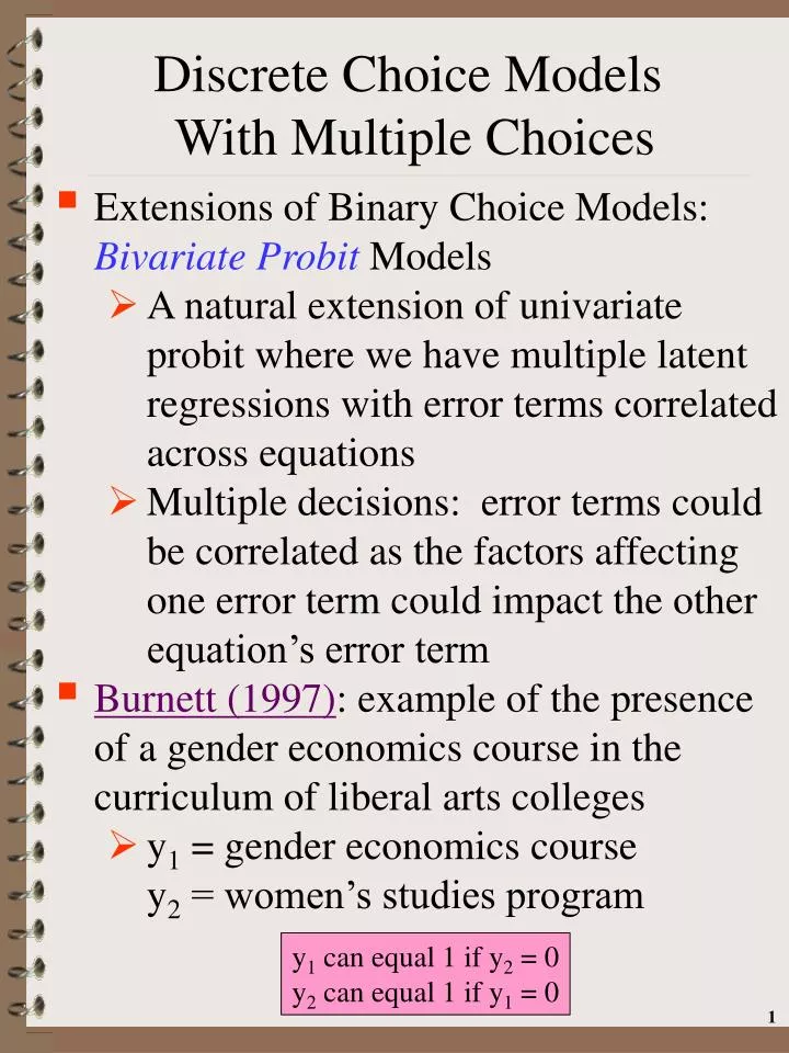
Discrete Choice Models With Multiple Choices. Extensions of Binary Choice Models: Bivariate Probit Models A natural extension of univariate probit where we have multiple latent regressions with error terms correlated across equations

E N D
Discrete Choice Models With Multiple Choices • Extensions of Binary Choice Models: Bivariate Probit Models • A natural extension of univariateprobit where we have multiple latent regressions with error terms correlated across equations • Multiple decisions: error terms could be correlated as the factors affecting one error term could impact the other equation’s error term • Burnett (1997): example of the presence of a gender economics course in the curriculum of liberal arts colleges • y1 = gender economics course y2 = women’s studies program y1 can equal 1 if y2 = 0 y2 can equal 1 if y1 = 0
Discrete Choice Models With Multiple Choices • General specification for a 2 equation model with error terms having a standard normal distribution: Latent variables X1 is (T x K1) X2 is (T x K2) K1 may not = K2 = error term correlation coefficient across equations given assumption that σ2ε= 1 Error term cov. matrix
Discrete Choice Models With Multiple Choices • There are four combinations of observed values of y1 and y2 → four probabilities • Remember the following latent relationships and mappings to observed y1 = 0 if y1*≤ 0→X1β1 + ε1 ≤ 0→ε1 ≤ −X1β1 y1 = 1 if y1*> 0→X1β1 + ε1 > 0→ε1 > −X1β1 y2 = 0 if y2*≤ 0→X2β2 + ε2 ≤ 0→ε2 ≤ –X2β2 y2 = 1 if y2*> 0→X2β2 + ε2 > 0→ε2 > –X2β2 3
Discrete Choice Models With Multiple Choices • Given the above mappings from yj* to yj • The above error term relationships imply P(y1=0,y2=0) = Pr(ε1 ≤ –X1β1, ε2 ≤–X2β2) P(y1=1,y2=1) = Pr(ε1 > –X1β1, ε2 >–X2β2) P(y1=0,y2=1) = Pr(ε1≤ –X1β1, ε2>–X2β2) P(y1=1,y2=0) = Pr(ε1 > –X1β1, ε2 ≤ –X2β2) • Now lets look at one particular functional form for the joint probability distribution of the two error terms 4
Discrete Choice Models With Multiple Choices • In general, the bivariatestandard normal CDF for two RV’s z1 and z2 is Definition of Bivariate Std. Normal PDF zj ~ N(0,1) correlation coefficient No. of RV’s z1, z2 cov. matrix
Discrete Choice Models With Multiple Choices • MATLAB Command for a bivariate normal CDF: p=mvncdf (X,μ, Σ)where • X is an T x 2 matrix of upper limits of integration • μ is a (1 x 2) vector • Σ is a (2 x 2) covariance matrix • Standard normal: • Order of integration automatically set by the number of columns in X • Each column represents a standard normal random variable • Zero means • Unitary variances • Covariance = correlation = ρ where −1 ≤ ρ≤ 1
Discrete Choice Models With Multiple Choices Pr(x,y) Here X and Y are 2 RV’s Pr(y|x)
Discrete Choice Models With Multiple Choices • Returning to our latent regression model • With the assumption of bivariate standard normal errors we have Note: Φ2(•) indicates 2 dimension standard normal CDF, P(ε2 > –X2β) = P(ε2≤ X2β) and the change of sign in ρ • We can use the above bivariate standard normal CDF to generate the LLF for the bivariate probit model • Four sets of integration limit pairs • Depends on the four combinations of our observed data, y1 and y2 8
Discrete Choice Models With Multiple Choices • To develop the log-likelihood function lets introduce some notation • i identifies observation j identifies choice • Similar to the univariate case • qij≡ 2yij−1 • qij = 1 if yij= 1 • qij= −1 if yij= 0 • Zij ≡ Xijβj • Wij≡ qijZij • ρi*≡ qi1qi2ρ • If one of the choices not made than ρi* = −ρ • If both choices either 1 or 0 then no change in sign, ρi* = ρ • Only oneρ coefficient estimated as sign change is based on data j=1,2 i=1,…,T qij=+1,-1 yij is observed Note: βvaries by choice and could be of different dimension for other j’s Wij is either Xijβj or –Xijβj 9
Discrete Choice Models With Multiple Choices • From the above joint PDF we have: Pr(y1=yi1,y2=yi2|Xi1,Xi2)=Φ2(Wi1,Wi2,ρi*) • The above accounts for sign changes associated with the 4 combinations of ones and zeros for the two y values • Pr(0,0|X1,X2) Pr(1,0|X1,X2) Pr(0,1|X1,X2) Pr(1,1|X1,X2) Bivariate Standard Normal CDF Zij=XijβjWij≡qijZij ρi* ≡ qi1qi2ρqij ≡ 2yij−1
Discrete Choice Models With Multiple Choices • From the above joint std. normal PDF: Pr(y1=yi1,y2=yi2|X1,X2)=Φ2(Wi1,Wi2,ρi*) • Given the definition of the sample likelihood function, this implies the sample LLF can be represented as: • L(β1,β2,ρ|X1,X2,y1,y2) = ΣilnΦ2(Wi1,Wi2,ρi*) • MATLAB Command • Bi_Prob=mvncdf(big_W,mu_0,Sigmai*) • where mu_0 is (1 x 2) vector or zeros • big_w is (T x 2) matrix of cdf arguments Bivariate Standard Normal CDF Zij=XijβjWij≡qijZij ρi* ≡ qi1qi2ρqij ≡ 2yij-1 11
Discrete Choice Models With Multiple Choices • Note that for the above we have: 12
Discrete Choice Models With Multiple Choices • The K1+K2+1 FOC’s for maximizing the above LLF can be represented via: K1+K2+1 due to ρ Zij=XijβiWij≡qijZij ρi* ≡ qi1qi2ρ qij ≡ 2yij-1 Univariate Std. Normal CDF Univariate Std. Normal PDF
Discrete Choice Models With Multiple Choices • ML estimates are obtained by setting the three sets of derivatives to 0. • When ρ = 0→independent error terms • FOC reduce to the univariate probit results for each yj • The total LLF would be the sum of 2 univariate probit LLF’s • →you simply estimate each probit separately and then add LLF values • Greene (p. 819) provides an overview of the 2nd order derivatives (and Hessian) • As he states, “…The complexity of the 2nd derivatives for this model makes it an excellent candidate for the BHHH estimator of the variance of the ML estimator”
Discrete Choice Models With Multiple Choices • As usual, we can use the Wald, Lagrange Multiplier and Likelihood Ratio tests to test the null hypothesis of zero correlation (H0: ρ=0) • Wald test is simply the square of the estimate of rho divided by its variance • Likelihood ratio test is two times the difference of the unrestricted LLF and the sum of the univariate probit LLF’s: LLR=2[LLFT – LLFy1 – LLFy2] Bivariate Std. Normal LLF univariate probit LLF’s Restricted model assumes independent error terms that are not correlated, ρ=0 15
Discrete Choice Models With Multiple Choices • Lagrange Multiplier test of the null hypothesis of zero correlation (H0: ρ=0) • One can calculate a LM test statistic based on univariate standard normal PDF’s and CDF’s (Greene p. 820): • All one needs to do is estimate univariate probits with no need to calculate bivariate probit Zij=XijβiWij≡qijZij ρi* ≡ qi1qi2ρ qij ≡ 2yij-1 Restricted Model assumes no correlation, i.e. ρ=0 16
Discrete Choice Models With Multiple Choices • Lets now talk about marginal effects under the bivariate probit model • Given that there may be different variables in X1 and X2 we will define the matrix X as their union: X ≡ X1 X2 • Also let X1β1=Xγ1 where γ1 contains all elements of β1 and 0’s in the position of variables in X that appear only in the X2 • Similar definition for γ2: 0’s in the position of variables in X that appear only in X1 → X2β2=Xγ2
Discrete Choice Models With Multiple Choices • Defining the joint probability that both y1 and y2 are 1 in terms of X, γ1, γ2: Pr(y1=1,y2=1|X) = Φ2(Xγ1,Xγ2,ρ) • Signs are changed if a 0 value is desired for one (both) of the yi’s • Pr(y1=0,y2=0|X) = Φ2(−Xγ1,−Xγ2, ρ) • Pr(y1=0,y2=1|X) = Φ2(−Xγ1,Xγ2, −ρ) • Pr(y1=1,y2=0|X) = Φ2(Xγ1, −Xγ2, −ρ)
Discrete Choice Models With Multiple Choices • The marginal effect of a change in X on the above joint probabilities can be obtained from the following: and • If ρ = 0 we obtain the univariate results • Φ2(Wi1,Wi2,ρi*) = Φ (Wi1)Φ(Wi2) Varies across 0,1 pairs Zij=Xijβj Wij≡qijZij ρi* ≡ qi1qi2ρ qij≡ 2yij-1 j = 1,2 Via product rule 19
Discrete Choice Models With Multiple Choices • Similar to the CRM and the univariate discrete choice situation, we have the following expectations: • Unconditional expectation continues to be: E(yj)=Φ(Xγj) (j = 1,2) • Previous univariate marginal analysis applies: • Conditional Expectation: E(y1|y2=1) Via chain rule conditional probability E[y1|y2=1,X]
Discrete Choice Models With Multiple Choices • The marginal effects of this conditional probability is: • More generally (above was for y2 = 1): • Partial derivatives of the above are the same as the first example with sign changes in several places when y2 = 0 gj defined above q2=2y2−1
Discrete Choice Models With Multiple Choices • Credit card application example • 1319 observations on applicants for a major credit card • y1 ≡ 1 if applicant had a major derogatory credit history report (MDR) • MDR defined as a delinquency of 60 days or more on a credit account • y2≡ 1 if an application for a credit card was accepted (Accept) L = ΣilnΦ2(Wi1,Wi2,ρi*)
Discrete Choice Models With Multiple Choices • Cross-tabulation of y1 (MDR) and y2 (Accept) • Distribution of Observations • y1 = 1 (MDR): 19.6% • y2 = 1 (Accept): 77.6% • y1 = y2 = 1: 8.2% • y1 = y2 = 0 = 11.0% Accept MDR 42% Accept=1|MDR=1 49% No MDR|Accept=0
Discrete Choice Models With Multiple Choices • Explanatory Variables • X1(MDR): Constant, Age, Income, Average Monthly Credit Card Exp. • X2 (Accept): Constant, Age, Income, Own Home(0/1), Self-Employed (0/1) 24
Discrete Choice Models With Multiple Choices • We showed earlier that the gradient vector of the LLF for the β’s is • What if the program during the optimization process wants to make an intermediate estimate of ρ>1 or < −1? 25
Discrete Choice Models With Multiple Choices • We need to develop some way for not allowing this to happen • How can we guarantee that the allowable search space will limit possible values of ρ to be in the range: −1 ≤ ρ≤ 1? • At the same time, this system needs to be differentiable 26
Discrete Choice Models With Multiple Choices • We use the TANH function to guarantee that the |ρ| ≤ 1. • MATLAB command: rho = tanh(b(totparm)) • Calculated ρ coefficient is −0.713 • Use a separate function to determine estimated ρ variance via delta method • Estimated std. error for ρ is 0.036 Parameter actually estimated ρ Nonlinear function of a coefficient βρ Est. coefficient used as input Function [est_rho]=Define_rho(b) ; est_rho = tanh(b(totparm)); end;
Discrete Choice Models With Multiple Choices • The following provides a flowchart of the MATLAB code used to estimate the bivariate probit model • The numerical BHHH estimation algorithm is used 28
Discrete Choice Models With Multiple Choices Exogenous Variables MDR, Accept 2 CRM’s Analytic Gradient and Hessian Probit LF Starting Values Univariate Probits NR Alg. Likelihood Functions Starting Values Bivariate Probit LF Numeric Gradient and Hessian Bivariate Probit tanh used to estimate ρ BHHH Alg. Likelihood Function Test for Correlation: H0:ρ=0 Coefficients & Covariance Matrix Determine ρ variance
Discrete Choice Models With Multiple Choices • Example of credit card application • y1 ≡ 1 if applicant had a major derogatory history report (MDR) • y2≡ 1 if application for a credit card was accepted (Accept) • From above we have defined the sample log-likelihood (L) for the bivariate probit model as: L=Σiln Φ2(Wi1,Wi2,ρi*) Wij ≡ qijXijβj ρi*≡ qi1qi2ρ qij=2yij-1 30
Discrete Choice Models With Multiple Choices • We undertake a variety of asymptotic χ2 test statistics of independence of events • Wald Statistic • Likelihood Ratio • Lagrangian Multiplier (Greene, p. 820) Zij=Xijβj Wij≡qijZij qij≡ 2yij-1 31
Discrete Choice Models With Multiple Choices • Calculate the marginal effects of changes in exogenous variables • Unconditional joint probability Pr(y1=1,y2=1|X) = Φ2(Xγ1,Xγ2,ρ) • Conditional probability 32
Discrete Choice Models With Multiple Choices • Lets now talk about the situation where there is a single decision to be made where that decision involves more than two choices that are mutually exclusive • Contrast this to the bivariate probit situation where we have two decisions each with a 0/1 value • Example of commute mode choice: Bus, train, car, bicycle or walking • These choices are unordered • Unordered choice models can be motivated by random utility where the ith consumer faces J+1 choices Uij = Zijβ + εijwhere Z are exog. variables • If ith agent makes choice j then this implies that Uij is the maximum among the J+1 utilities
Discrete Choice Models With Multiple Choices • The statistical model is based on the result that choice j is made if Pr(Uj>Uk) for all k ≠ j is the largest • Model is operationalized by assuming a particular utility function error term distribution • With J+1 fairly large one would need to evaluate J+1 integrals under the normal distribution (PDF) • i.e., think about the likelihood function under the bivariate probit • → the probit model is not usually used with many choices • In contrast, the logit model uses an error term distribution functional form that allows for a relatively large number of choices
Discrete Choice Models With Multiple Choices • Using the notation of McFadden (1973), suppose an individual faces J+1 choices • Lets define an underlying latent variable Uj* to represent the level of indirect utility associated with the jth choice • There may be errors in the utility maximization process because of • Imperfect perception • Imperfect optimization or • Inability of the analyst to measure exactly all relevant variables • →Latent utility is our random variable • The observed variable, yjis defined as: (assuming there are no ties) J+1 choices
Discrete Choice Models With Multiple Choices j is choice i is individual • Let Uij*=Uij (Xij, Wi) + εij ( j = 0,1,…,J) (i = 1,…,T) • Wi’s are individual specific characteristics (don’t change across j) • Xij’s are attributes of the jth choice as perceived by the ith individual • e.g. travel time from your house via a particular travel mode • εij is a residual that captures unobserved • variations in tastes • attributes of alternatives • errors in consumer’s perception and optimization • Assume residuals are IID with Type I Extreme Value distribution: • CDF: F(εj < ε*) = exp(−e−ε*) • PDF: f(εj) = exp(−εj− e−εj) Note: εij not impacted by εkj
Discrete Choice Models With Multiple Choices • The above decision rule implies that if choice j is made then (omitting i subscript): Uj + εj > Uk + εk for k ≠ j → εk < Uj + εj– Uk for k ≠ j • This implies • If εj is considered given, this expression is the CDF for each εk evaluated at εj+Uj–Uk • As noted above, if the error terms are IID extreme value this CDF is • Since the errors are independent, the CDF over all k ≠ j is the product of the individual CDF’s choices CDF: F(εj < ε*) = exp(-exp(-ε*))
Discrete Choice Models With Multiple Choices Joint probability • Of course εj is not given, so the choice is the integral of the above conditional probabilities over all values of εj weighted by its density • As shown by Train (p. 78-79, 2003) and McFadden(1977) given the above we have: PDF of εj, Type I Extreme Value This is why we like to use this funcitonal form 38
Discrete Choice Models With Multiple Choices • Representative utility is usually specified to be linear in parameters • McFadden(1973) shows iff the J+1 error terms are iid with type 1 extreme value (Gumbel) distribution • The above is known as the conditional logit ( or sometimes multinomial but be careful there is a difference) model • Note that the β’s do not vary across choice Zij are exog. variables Uij=Zijβ j is choice i is individual J + 1 Choices 39
Discrete Choice Models With Multiple Choices • As in the bivariate choice environment, the exogenous variables Z are composed of variables specific to the individual as well as the choices: Zij=[Xij Wi] • Xij varies across choices and possibly across individuals and referred to as choice attributes • Wi contain characteristics of the individual which are the same across choices (e.g., an individual’s age) • Why is it important that we distinguish between these two types of variables?
Discrete Choice Models With Multiple Choices • Incorporating the above in the definition of the conditional logit model: • → factors that do not vary across choice (e.g., specific to the individual) fall out of the above probability • To allow for individual specific effects the model needs to be modified • One method is to create a set of dummy variables for each of the J+1 choices • Multiply by the common W where one of the interactions is dropped Uij=Zijβ* j is choice i is individual
Discrete Choice Models With Multiple Choices • Using the example of Greene (p.843) with 3 choices as to what shopping center to use: • The choice dummy times the income variable places a “j” subscript on W → the numerator and denominator terms will not cancel each other • Resulting model: Cj is shopping center dummy
Discrete Choice Models With Multiple Choices • Resulting model: • α1 and α2 coefficients associated with dummy weighted income values • Interpreted as the income effect relative to omitted category (choice 3 in this example) Note no intercept 43
Discrete Choice Models With Multiple Choices • As under the univariate discrete choice models, the coefficients are not the marginal effects of attribute changes Using the notation of Train Vij ≡ Xijβ Xij is a vector Effect of own X on ownprobability Due to quotient and chain rule Effect on carprob. of a change in car commute time 44
Discrete Choice Models With Multiple Choices =1 when j = n, 0 otherwise • This can be easily extended to otherchoice attributes (Xn) effects on the jth probability • Given that Pj and Pn are in the above marginal effects, every attribute set affects all probabilities given the conditional logit denominator • To see this, we have the following: j≠n, effect on carprob. of a change in train commute time j,n are two choices Via chain rule 45
Discrete Choice Models With Multiple Choices quotient rule Pij Pin Pij 46
Discrete Choice Models With Multiple Choices • The elasticity of a change in attribute k of choice n on Pj (Γknj) at a particular point can be represented as: (1x1) j,n are choices k is an attribute 47
Discrete Choice Models With Multiple Choices • As noted by Train(2003) p. 64, with respect to the cross elasiticities on the jth probability of the nth choices attributes: • A change in an attribute of alternative n changes the jth probability (j≠n) for other alternatives by the same percent • No ”j” in the above elasticities • This is a restatement of the Independence from Irrelevant Alternatives(IIA) characteristic of logit choice probabilities we will discuss later j,n are choices k is attribute 48
Discrete Choice Models With Multiple Choices • The sample log-likelihood for the conditional model can be derived by defining the variable dij = 1 if alternative j is chosen by individual i, 0 otherwise for the J +1 possible outcomes • For a particular individual, only 1 of the dij’s is non-zero (→Σjdij=1) • The total sample log-likelihood is a generalization of the likelihood function for the binomial logit or probit model: Pij Again no j subscript for estimated coeff. 49
Discrete Choice Models With Multiple Choices • We can provide an alternative form of the totalsample log-likelihood function: Previous Result This is what I use in my MATLAB code 50