Download
1 / 28
280 likes | 419 Vues
Reconstructing Phylogenies from Gene-Order Data. Overview. What are Phylogenies?. “Tree of Life” A UAG representing evolution of species. Phylogenic Analysis Used For…. Phylogenies help biologists understand and predict: functions and interactions of genes genotype => phenotype

E N D
What are Phylogenies? • “Tree of Life” • A UAG representing evolution of species
Phylogenic Analysis Used For… • Phylogenies help biologists understand and predict: • functions and interactions of genes • genotype => phenotype • host/parasite co-evolution • origins and spread of disease • drug and vaccine development • origins and migrations of humans • RoundUp herbicide was developed with the help of phylogenetic analysis
Gene-Level Phylogeny • Nadeau-Taylor model of evolution • Assume discrete set of genes • Each gene represents a sequence of nucleic acids • Genes have polarity (a, -a) • A species genome is a sequence of genes • Rare evolutionary events cause changes in genome • Inversion: (a b c d) => (a –c –b d) • Transposition: (a b c d) => (a c d b) • Inverted transposition: (a b c d) => (a –d –c b) • Insertion: (a b c d) => (a e b c d) • Deletion: (a b c d) => (a c d)
Goal of Phylogenetics • Given a set of observed genomes, reconstruct an evolutionary tree • Leaves are the observed genomes • Internal nodes are evolutionary steps (“missing link” genomes) • Edges may contain multiple events • Fundamentally impossible to solve without a time machine • Fossils? • However: • Of the set of valid trees that include all observed genomes as leaf nodes, tree containing the minimum number of events (sum of edge weights) is closest to actual • “Maximum parsimony”
Tree Construction Techniques • Three primary methods: • Criterion-based (NP-HARD optimization) • Relies on an evolutionary model • Examples: • Breakpoint phylogeny • Maximum-likelihood, maximum-parsimony, minimum evolution • Provides good accuracy but intractable for larger sets of genomes • Ad hoc / distance-based • Relies on pair-wise distances • Example: • Neighbor-joining • Runs in polynomial time but very inaccurate for large sets of genomes • Meta-methods • Ex: disk-covering, quartet-based methods • Divide-and-conquer approach
Breakpoint Phylogeny Method • Sankoff-Blanchette Technique • Assume an unrooted, binary tree topology, where leaves are genomes • Basic algorithm: • For each circular ordering of genomes… • From bottom up, label each of the 2N-2 internal nodes with a genome that has minimal distance to each of its neighbors • The tree with the minimal sum of edge-weights (height) is the most parsimonious • First problem with S-B: exponential number of genome orderings (n-1)! possible circular orderings: G1 G2 G3 G4 is equivalent to… G2 G3 G4 G1 Topology (and thus length) of tree depends solely on gene ordering
Breakpoint Distance • S-B use “breakpoint distance” to estimate distance between two genomes • Approximates number of evolutionary events • Assumes consistent gene set and sequence length • Given genomes G1 and G2 • If a and b are adjacent in genome G1 but not in G2, then bp_distance++ • Example: {a b c d} and {a c d b} have two breakpoints • Must also take polarity into account… • No breakpoint between {a b} and {-b –a} • Example: {a b c d} and {-b –a c d} • Breakpoint distance is 1
“Median Problem for Breakpoints” • S-B labels internal nodes by finding a median among 3 genomes, such that: • D(S,A) + D(S, B) + D(S,C) is minimal • Performed using a TSP: • Build fully-connected graph with an edge for each polarity of each gene • Edge weights assigned as 3-(number of times each pair of genes are adjacent) • Run TSP • Path of salesman specifies medium
-D D A -A C -C B -B Example Median • Assume gene set={A, B, C, D} • Assume genomes: A B C D B D -A -C -D C B A u(A,B)=0 u(A,-B)=1 u(A,C)=0 u(A,-C)=1 u(A,D)=0 u(A,-D)=0 u(-A,B)=1 u(-A,-B)=0 u(-A,C)=0 u(-A,-C)=0 u(-A,D)=0 u(-A,-D)=1 u(B,C)=0 u(B,-C)=1 u(B,D)=0 u(B,-D)=0 u(-B,C)=1 u(-B,-C)=0 u(-B,D)=1 u(-B,-D)=0 u(C,D)=1 u(C,-D)=0 u(-C,D)=1 u(-C,-D)=0 2 weight=3-(adjacencies) -1 If solution to TSP is s1,-s1,s2,-s2,…,sn,-sn then median is s1,s2,…,sn (include signs) 2 2 2 -1 -1 2 2 2 2 -1 2 edges not shown have weight 3
S-B Algorithm N+2N-2 label initialization only when nodes have changed
S-B Algorithm • S and B propose three different methods for initializing the TSPs for achieving global optimum • Second problem with S-B: • Each tree requires the solving of multiple TSPs, which themselves are NP-HARD • Initial labeling: 2N-2 TSPs • Repeats this process an unknown number of times to optimize internal nodes
Neighbor Joining • A polynomial-time heuristic for tree construction • Given the distances between each pair of genomes (distance matrix)… • Grow a complex tree structure, starting from a star • Basic algorithm: • Begin with a star-topology • Choose pairs of leaves that are closely related • Remove these leaves and join them with a new internal node • Join this new internal node somewhere into the old tree • Do this until all N-3 internal nodes have been created
X 1 2 3 5 4 1 2 X Y 3 4 5 Neighbor-Joining N(N-2)/2 possibilities S0=(S D)/(N-1) = 45/4 = 11.25
Neighbor-Joining • Edges weight approximations can be computed with neighbor-joining • However, it is more accurate to label the internal nodes as with S-B and measure edge lengths based on this • “Scoring”
Moret’s Distance Estimators • IEBP estimator • Approximates event distance from • breakpoint distance • weights: inversion, transposition, inverted transposition • Fast but not accurate • Exact-IEBP • Returns the exact value • Slow but exact • EDE • Correction function to improve accuracy of IEBP • EDE used to build distance matrix • Set up NJ • Finding lower bound • Scoring
EDE • Distance correction • Non-negative inverse of • F(x) defines minimum inversion distance, x defines actual inversions
Bounding • Given a distance matrix, lower bound can be determined • “Tree is at least this size” • Use “twice around the tree” • Length of tree (sum of edges) is .5 * (d12, d23, …, dn1) • Given a constructed tree, upper bound can be determined • Label internal nodes • Sum up all edges using distance calculator
GRAPPA • Optimizations • Gene ordering • Given a circular gene ordering • Build a S-B tree • Swap internal leaf orderings, changing the order • Upper bound stays constant (no relabeling), while lower bound changes
GRAPPA • Layered search: • Build EDE distance matrix • Build and score NJ tree (provides initial upper bound) • Enumerate all genome orderings • For each: • Compute lower bound using “twice around the tree” • If LB < UB, add ordering to queue, sorted by LB • Requires too much disk space • Score each tree from queue in order: • Keep track of lowest upper bound • Allows for more pruning
GRAPPA • Without layered search: • Build EDE distance matrix • Build and score NJ tree (initial upper bound) • For each genome ordering: • Compute lower bound • If lower bound < UB • Score tree and compute new upper bound (may do swap-as-you-go to eliminate redundant orderings) • If new upper bound < old upper bound, set new upper bound
FPGA Implementation • Software can perform NJ, since that’s only done once • Software can enumerate valid genome orderings • Scoring should be done in hardware • EDE can be performed via BRAM/CLB lookup table • Need to implement TSP in hardware • GRAPPA uses specialized version of TSP • As opposed to chained and simple versions of Lin-Kernighan heuristic – O(n3) • Most important question: • Map to multi-FPGA architecture?
GRAPPA Version of S-B Algorithm • Iterative refinement • Only refine internal nodes when one of the neighbors has changed in the refinement iteration • Condenasation • Gene reduction to speed up TSP for shared subsequences • Not used by default • Exact TSP algorithm • Initial labeling • Uses second approach in S-B paper (“nearest neighbors/trees of TSPs”)
Parallelism? • Scoring is very parallel • TSP only depends on three nearest nodes • Can overlap iterations • GRAPPA is parallelized for cluster • Compute, not communication bound • Achieve finer-grain parallelism with FPGAs • Problem may turn communication-bound • Research Plan • GRAPPA analysis (drill-down) • Get preliminary results for TSP over FPGA • SRC implementation (Charlie) • Determine granularity vs. communication
I4 I5 I3 I2 I1 I6 G3 G2 G1 G4 Possible HPRC Approach I1 I2 I3 I4 I5 I6 wrap-around – one TSP core buffered requests
Possible HPRC Approach input species ancesteral group 1 ancesteral group 2 g5 g5 g5 g5
HPRC • FPGAs • Comp. density • Cost • Granularity • Mesh • Load balancing