Download
1 / 40
460 likes | 962 Vues
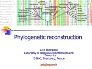
I519 Introduction to Bioinformatics, 2012. Phylogenetic Tree Reconstruction. Evolution theory. Speciation Evolution of new organisms is driven by Mutations The DNA sequence can be changed due to single base changes, deletion/insertion of DNA segments, etc. Selection bias

E N D
I519 Introduction to Bioinformatics, 2012 Phylogenetic Tree Reconstruction
Evolution theory • Speciation • Evolution of new organisms is driven by • Mutations • The DNA sequence can be changed due to single base changes, deletion/insertion of DNA segments, etc. • Selection bias • Speciation events lead to creation of different species. • Speciation caused by physical separation into groups where different genetic variants become dominant • Any two species share a (possibly distant) common ancestor • The molecular clock hypothesis • Indiana University (Michael Lynch, Jeff Palmer, Matt Hann et al) Lynch: The Origins of Genome Complexity
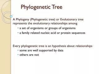
Aardvark Bison Chimp Dog Elephant Phylogeny (phylogenetic tree) • A phylogenetic tree is a graph reflecting the approximate distances between a set of objects (species, genes, proteins, families) in a hierarchical fashion taxon • Leaves – current species; sequences in current species • Internal nodes - hypothetical common ancestors • Branches (Edges) length - “time” from one speciation to the next (branching represents speciation into two new species)
Phylogenetic trees (binary trees) Rooted tree Rooted tree satisfying “molecular clock” hypothesis: all leaves at same distance from the root. root 6 root 7 8 time 7 6 8 3 5 1 2 UMPGA 4 1 2 3 4 5 Unrooted tree: Note: 1-5 are called leaves, or leaf nodes. 6-8 are inferred nodes corresponding to ancestral species or molecules. Branches are also called edges. The edge lengths reflect evolutionary distances. 3 4 8 6 2 7 5 1
Morphological vs. molecular • Classical phylogenetic analysis: morphological features: presence or absence of fins, number of legs, lengths of legs, etc. • Modern biological methods allow to use molecular features • Gene sequences • Protein sequences • Species tree and gene tree
From sequences to phylogenetic tree Rat QEPGGLVVPPTDA.. Rabbit QEPGGMVVPPTDA.. Gorilla QEPGGLVVPPTDA.. Cat REPGGLVVPPTEG.. There are many possible types of sequences to use (e.g. Mitochondrial vs Nuclear proteins).
How to choose the best tree? • To decide which tree is best we can use an optimality criterion. • Parsimony is one such criterion (the other criteria: Maximum likelihood, minimum evolution, bayesian) • It chooses the tree which requires the fewest mutations to explain the data. • The Principle of Parsimony is the general scientific principle that accepts the simplest of two explanations as preferable.
AAA AAA 1 AAA AAA AGA AAA 1 2 1 1 1 AAA AGA AGA GGA AAG GGA AAG AAA Total #substitutions = 3 Total #substitutions = 4 Principle of Parsimony Parsimony based methods look for a tree with the minimum total number of substitutions of symbols between species and their ancestor in the phylogenetic tree. The left tree is preferred over the right tree.
Maximum parsimony A C C A S1 CACCCCTT S2 AACCCCAT S3 CACTGCTT S4 AACTGCTA (S1,S2),(S3,S4) 20011011 6 (S1,S3),(S2,S4) 10022011 7 S2 S1 S3 S1 C A C C C A S2 mutation=2 (S1,S2), (S3, S4) mutation=1 (S1,S3), (S2, S4) C A A A S4 S4 S3
We can EASILY get different trees (the “reality check” paper) • Input sequences • Multiple alignment programs • Substitution models • Phylogenetic tree reconstruction methods
Trees – what might they mean? Species A Species B Species tree Species C Species D Seq A Gene tree Seq D Seq C Seq B
Weak support, 40% bootstrap for bipartition (AD)(CB) Lack of resolution Seq A Seq D Seq C Seq B (typical >80%)
the two longest branches join together Strong support, e.g., 100% bootstrap for (AD)(CB) Long branch attraction (LBA) Seq A Seq D Seq C Seq B
Gene Transfer Seq A Seq D Seq C Seq B speciation genetransfer Horizontal gene transfer species A species B Species tree species C species D Gene tree
Seq A Seq B Seq C Seq D Seq B’ Seq C’ Seq D’ species A Gene duplication & loss Species tree species B species C Duplication species D Loss Gene tree A D C B
Orthologs and paralogs (important for function annotation) Seq A • Orthologs: • sequences diverged after a speciation event • Paralogs: • sequences diverged after a duplication event • Xenologs: • sequences diverged after a horizontal transfer Seq B SeqC Seq D gene duplication Seq B Seq C Seq D Duplicated genes may have different functions!!
Phylogeny (phylogenetic tree) reconstruction: overview • Tree topology & branch lengths • Computational challenge • Huge number of tree topology 3 sequences: 1 (unrooted) 4 sequences: 3 5 sequences: 15 10 sequences: 2,027,025 20 sequences: 221,643,095,476,699,771,875 n sequences (unrooted & rooted) ?? • Most methods are heuristic • Two types of methods • Distance based (input: distance matrix; UPGMA & NJ) • Character based (input: multiple alignment)
Models of evolutionary distance A G C T 1. Simplest case: Jukes-Cantor model -- equal probability of change to any nucleotide 2. Other models take into account transitions vs. transversion frequencies -- Kimura: different probabilities for transitions, transversions -- HKY: different probabilities for transitions, transversions & takes into account genomic nucleotide biases Transition: R to R Y to Y Transversion: R to Y Y to R where R = A,G Y = C,T b b
A a C c b B Distance based phylogeny reconstruction • Phylogeny reconstruction for 3 sequences is EASY • There is a single tree topology • The branch lengths can be calculated as follows: To compute: branch lengths a, b and c, such that Input: DAB, DBC and DAC (pairwise distances) Output:
Fitch-Margoliash (FM) algorithm • For phylogeny reconstruction with more than 3 sequences • For example, given 5 sequences, A, B, C, D and E. The tree can be reconstructed as follows • First choose the closest sequence pair, suppose it is D and E (based on the input pairwise distances; e.g., DDE=10) • To calculate the branch lengths from D and E to their common ancestor (denoted as d and e), we combine the remaining three sequences (A, B and C) and treat them as a single composite sequence (and define and so on) -- so again we are dealing with 3 sequences, and we can easily calculate the branch lengths • Then merge D and E into a cluster and treat it as a composite sequence, and update the distance table so that and so on. • Repeat the above steps until no more clusters to merge
Distance based method: UPGMA • UPGMA: Unweighted Pair Group Method with Arithmetic Mean • Assume same rate evolution (molecular clock hypothesis) • The length from root to each leaf is the same (ultra metric). • It is similar to Fitch-Margoliash algorithm (merge two most similar sequences or clusters first); but the calculation of branch lengths is even simpler. • For example, for the same example shown above with five sequences, d=e=5 (d and e are the branch lengths from sequence D and E to their common ancestor)
Neighbor-joining (NJ) (Seitou & Nei algorithm) • Minimum evolution -- the least total branch length (distance-based) • Bottom-up clustering method • Does not assume same rate evolution • Fast & produce reasonable trees
NJ method 3 3 2 2 4 4 X Y X 1 1 5 5 NJ looks for two sequences (clusters) to merge that minimizes: Where C1 and C2 are most similar to each other, while they are most dissimilar to the other clusters (far from others)
Comparison of FM, UPGMA and NJ methods • All are hierarchical clustering methods • All define the distance between two clusters as the average pairwise distance • FM and NJ do not assume “molecular clock”; UPGMA does and it uses a simpler way to calculate branch lengths. • UPGMA and FM choose and merge the closest sequence (cluster) pair first, but NJ looks for two sequences (clusters) that are not only close to each other (as in UPGMA and FM) but also far apart from the rest
Parsimony based reconstruction • A procedure to find the minimum number of changes needed to explain the data for a given tree topology, where species are assigned to leaves. (Small Parsimony Problem) • A search through the space of trees. (hard problem!) (Large Parsimony Problem)
Small Parsimony Problem • Compute the minimum number of mutations on a GIVEN tree • Fitch algorithm • Sankoff algorithm (subtree; DP)
The Fitch Algorithm • Pick an arbitrary root to work towards (for unrooted tree) • Work from the tips of the tree towards the root. Label each node with the intersection of the states of its child nodes. • If the intersection is empty label the node with the union and add one to the cost TC T +1 +1 C C AGC +1 Cost=4 C +1 CT +1 GC C C CT= +1 +1 +1 C T G C A T C T G C A T Calculate Fitch score Internal node labeling
Sankoff Algorithm • More general than the Fitch algorithm. • Assumes we have a table of costs cabfor all possible changes between states a and b (A, T, C or G for DNA) • For each node i in the tree we compute S(i,a) the minimal cost given that node i is assigned state a. • In particular we can compute the minimum value over a for S(root,a) which will be the cost of the tree.
Sankoff algorithm: DP C T G A G T S(i,A) = S(i,T) = 0 S(i,G)=0 Initialization: S(i,a) = 0 i labeled by a, or S(i,a) = a{A,T,C,G} Iteration:S(i,a) = minx(S(j,x)+c(a,x)) + miny(S(k,y)+c(a,y)) Termination: minaS(root,a)
Large Parsimony Problem • The small parsimony problem – to find the score of a given tree - can be solved in linear time in the size of the tree. • The large parsimony problem is to find the tree with minimum score. • It is known to be NP-Hard.
Tree search strategies • Exact search • possible for small n only • Branch and Bound • Use “cleaver” rules to avoid some branches of trees • up to ~20 (25) taxa • Local search - Heuristics • Pick a good starting tree and use moves within a “neighbourhood” to find a better tree; e.g., nearest-neighbor interchanges (NNIs) • Meta-heuristics • Genetic algorithms • Simulated annealing
Branch and bound http://evolution.gs.washington.edu/gs541/2005/lecture25.pdf
Branch and bound This branch can be safely “neglected”!
Probabilistic approaches to phylogeny • Rank trees according to their likelihood P(data|tree), or, posterior probability P(tree|data) (Bayesian) • Maximum likelihood methods • Sampling methods
Calculate likelihoodFelsenstein’s algorithm for likelihood • Initialization: i=2n-1 • Recursion: Compute P(Li|a) for all a as follows if i is leaf P(Li|a)=1 if a is the label of the leaf, otherwise 0 else Compute P(Lj|a), P(Lk|a) for all a P(Li|a)=b,cP(b|a,tj)P(Lj|b)P(c|a,tk)P(Lk|c) i a k j b c
How can one tell if a tree is significant Biological knowledge Bootstrapping: how dependent is the tree on the dataset 1. Randomly choose n objects from your dataset of n, with replacement (picking columns from the alignment at random with replacement) 2. Rebuild the tree based on the subset of the data 3. Repeat many (1,000 – 10,000) times 4. How often are the same children joined? Jackknifing: how dependent is the tree on the dataset 1. Randomly choose k objects from your dataset of n, without replacement 2. Rebuild the tree based on the subset of the data 3. Repeat many (1,000 – 10,000) times 4. How often are the same children joined?
Commonly used phylogeny packages • 369 phylogeny packages (http://evolution.gs.washington.edu/phylip/software.html) and 54 free servers (as of Sep 30, 2011) • Phylip (general package, protdist, NJ, parsimony, maximum likelihood, etc) • PAUP (parsimony) • PAML (maximum likelihood) • TreePuzzle (quartet based) • PhyML (maximum likelihood) • MyBayes • MEGA (biologist-centric)
What a surprise • “..because of their intrinsic reliance on summary statistics, distance-matrixmethods are assumed to be less accurate than likelihood-basedapproaches. In this paper [Science, 327:1376–1379, 2010], pairwise sequence comparisons areshown to be more powerful than previously hypothesized. A statisticalanalysis of certain distance-based techniques indicates thattheir data requirement for large evolutionary trees essentiallymatches the conjectured performance of maximum likelihood methods—challengingthe idea that summary statistics lead to suboptimal analyses.”
Readings • Chapter 7 (Revealing Evolutionary History) • Chapter 8 (Building Phylogenetic Trees)