Supply Chain Management

1. Supply Chain Management Lecture 17

2. Outline • Today • Survey • Midterm • Brief semester overview • Start with Chapter 10 • Next week • Chapter 10 • 3e: Sections 1, 2 (up to page 273), 6 • 4e: Sections 1, 2, 3 (up to page 260)

3. Q1 Supply Chain Stages • A typical supply chain may involve a variety of stages Supplier Manufacturer Distributor Retailer Customer Most supply chains are actually supply networks

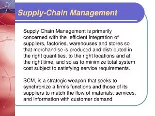
4. Q2 Push/Pull View of Supply Chain Processes Execution is initiated in response to customer orders (reactive) PULL PROCESSES Customer order arrives Execution is initiated in anticipation of customer orders (speculative) PUSH PROCESSES Processes are divided based on the timing of their execution relative to a customer order

5. Q3 Cycle View of Supply Chain Processes Customer Customer Order Cycle Cycle view defines the processes involved and the owner of each process Retailer Replenishment Cycle Distributor Manufacturing Cycle Manufacturer Procurement Cycle Supplier

6. Q4 Highly efficient Somewhat responsive Highly responsive Somewhat efficient Seven-Eleven Japan Most automotiveproduction Hanes apparel Integrated steel mills 2. Understanding the Supply Chain Capabilities • Supply chain capabilities • Supply chainresponsiveness • Respond to wide ranges of quantity demanded, meet short lead times, large variety, innovative products, high service level, etc • Supply chain efficiency (low cost)

7. Q5 1. Understanding the Customer and Supply Chain Uncertainty • Understanding customer uncertainty • Demand varies along certain attributes • Quantity in each lot, response time, variety of products needed, convenience, price, innovation, etc • Implied demand uncertainty • Demand uncertainty due to the portion of demand that the supply chain is targeting, not the entire demand

8. Q6 Key Observations • There is nosupply chain strategy that is always right • There is a right supply chain strategy for a given competitive strategy

9. Q7 Facilities Inventory Transportation Information Sourcing Pricing Logistical drivers Cross functional drivers From Strategy to Decisions Corporate Strategy Competitive Strategy Supply Chain Strategy Responsiveness Efficiency

10. Q8 Highly efficient Somewhat responsive Highly responsive Somewhat efficient Seven-Eleven Japan Most automotiveproduction Hanes apparel Integrated steel mills 2. Understanding the Supply Chain Capabilities • Supply chain capabilities • Supply chainresponsiveness • Respond to wide ranges of quantity demanded, meet short lead times, large variety, innovative products, high service level, etc • Supply chain efficiency (low cost)

11. Q9 Transportation Cost and Number of Facilities Transportation Costs Number of Facilities

12. Q10 Response Time and Number of Facilities Number of Facilities Response Time

13. Q11 Factors Influencing Distribution Network Design • Performance of a distribution network should be evaluated along two dimensions • Customer needs that are met (customer service) • Response time (Time it takes for a customer to receive an order) • Product variety (Number of different products that are offered) • Product availability (Probability of having a product in stock) • Customer experience (Ease of placing and receiving orders) • Order visibility (Ability of customers to track their orders) • Returnability (Ease of returning unsatisfactory merchandise) • Cost of meeting customer needs (supply chain cost) • Inventory (All raw materials, WIP, and finished goods) • Transportation (Moving inventory from point to point) • Facility & handling (Locations where product is stored, assembled, or fabricated) • Information (Data and analysis of all drivers in a supply chain)

14. Example: Retail stores such as Wal-Mart and JCPenney Customers pick up product from retailers Low transportation cost High facility cost Relative easy returnability Increased inventory cost No order tracking necessary If the product is available at the retailer, the consumer buys. Otherwise goes to another retailer Effective for fast moving items Q12 Manufacturers Distributor Warehouse Distributor Warehouse Retailer Retailer Retailer Consumers Retail Storage with Customer Pickup

15. Example: Amazon Inventory is held at a warehouse which ships to customer by carriers With respect to direct shipping Inventory aggregation is less Higher inventory costs Facility costs are higher Less information to track Warehouses are physically closer to consumers which leads to Faster response time Lower transportation cost Not effective for slow moving items Q13 Manufacturers Distributor Warehouse Distributor Warehouse Consumers Distributor Storage with Carrier Delivery

16. Example: eBags Products are shipped directly to the consumer from the manufacturer Retailer is an information collector: Passes orders to the manufacturers It does not hold product inventory Inventory is centralized at manufacturer Drop shipping offers the manufacturer the opportunity to postpone customization Effective for high value, large variety, low demand products High transportation cost Q14 Manufacturers Retailer Consumers Manufacturer Storage with Direct Shipping (Drop Shipping)

17. Q15 Inventory Cost and Number of Facilities Inventory Costs Number of Facilities

18. Q16 Logistics Costs Logistics Costs Facility Costs Transportation Costs Number of Facilities Total Logistics Costs Inventory Costs

19. Q17 Factors Influencing Network Design Decisions • Technological factors • Compare your supplies to the final product, considering whether value, weight, volume or other factors change • Availability of production technologies • High or low fixed cost • Semiconductor manufacturing takes place only in 5-6 countries worldwide (building one plant costs about 1 to 4 billion dollars) Which products gain/lose weight in the production process?

20. Q18 Factors Influencing Network Design Decisions • Political factors • Political stability • Infrastructure factors • Availability of transportation terminals, labor • Most of Amazon’s distribution centers are located near airports • Competitive factors • Positive externalities (many stores in a mall makes it more convenient for customers – one location for everything the customers need)

21. Q19 Factors Influencing Network Design Decisions • Technological factors • Compare your supplies to the final product, considering whether value, weight, volume or other factors change • Availability of production technologies • High or low fixed cost • Semiconductor manufacturing takes place only in 5-6 countries worldwide (building one plant costs about 1 to 4 billion dollars) Which products gain/lose weight in the production process?

22. Q20 Discounted Cash Flow Analysis • The present value of future cash is found by using a rate of return k • A dollar today is worth more than a dollar tomorrow • A dollar today can be invested and earn a rate of return k over the next period

23. Q21 Impact of Uncertainty in Network Design Supplier Manufacturer Distributor Retailer Customer Building flexibility into supply chain operations allows the supply chain to deal with uncertainty more effectively

24. Q22 Role of Forecasting Supplier Manufacturer Distributor Retailer Customer Push Push Push Pull Push Push Pull Push Pull Is demand forecasting more important for a push or pull system?

25. Q23 Summary: Simple Exponential Smoothing Method • Estimate level • The initial estimate of level L0 is the average of all historical data • L0 = (∑iDi)/ n • Revise the estimate of level for all periods using smoothing constant  • Lt+1 = Dt+1 + (1 – )*Lt • Forecast • Forecast for future periods is • Ft+n = Lt Forecast Ft+n = Lt

26. Q24 Types of Forecasts • Qualitative • Primarily subjective, rely on judgment and opinion • Time series • Use historical demand only • Causal • Use the relationship between demand and some other factor to develop forecast • Simulation • Imitate consumer choices that give rise to demand

27. Q25 Characteristics of Forecasts • Forecasts are always wrong! • Long-term forecasts are less accurate than short-term forecasts • Aggregate forecasts are more accurate than disaggregate forecasts • Information gets distorted when moving away from the customer

28. Q26 Time Series Forecasting Observed demand = Systematic component + Random component L Level (current deseasonalized demand) T Trend (growth or decline in demand) S Seasonality (predictable seasonal fluctuation) The goal of any forecasting method is to predict the systematic component (Forecast) of demand and measure the size and variability of the random component (Forecast error)

29. Q27 Aggregate Planning Strategies • Basic strategies • Level strategy (using inventory as lever) • Synchronize production rate with long term average demand • Swim wear • Chase (the demand) strategy (using capacity as lever) • Synchronize production rate with demand • Fast food restaurants • Time flexibility strategy (using utilization as lever) • High levels excess (machine and/or workforce) capacity • Machine shops, army • Tailored strategy • Combination of the chase, level, and time flexibility strategies

30. Q28 F6 = L5 L5 = (D5+D4+D3+D2)/4L5 = 292.75

31. Q29 F6 = L3 + 3T3 F5 = 125.0 Forecast Ft+n = Lt + nTt

32. Q30 APE1 = |E1/D1|*100 = 11.05 APE2 = |E2/D2|*100 = 4.26 MAPE2 = (APE1 + APE2)/2 = 7.65

33. Facilities Inventory Transportation Information Sourcing Pricing Overview • Chapter 10, 11, 12 • Inventory and product availability • Chapter 14, 15 • Sourcing and pricing Corporate Strategy Competitive Strategy Supply Chain Strategy Responsiveness Efficiency

34. High flexibility High cost Types of Inventory • Raw material inventory • Stocked at plant or supplier • Lowest cost • Work-in-process (WIP) Inventory • Raw materials transformed by operations • Need just enough • Finished-goods inventory • WIP after final operation • Stocked at plant, DC, retail store

35. The Importance of Inventory Every other time in the modern era that the U.S. economy has contracted more than 5% in a quarter, falling inventories have been a major reason, if not the single biggest factor. Usually, really bad recessions are worsened by the need for companies to get rid of all the stuff they made but nobody bought. Once the inventories are sold off, the economy can grow quickly again because idled workers are called back. But so far in this recession, the inventory cycle hasn't been a major factor, outside of the housing and auto sectors. … This recession is rooted in a severe credit squeeze and a fundamental readjustment in consumer demand, not in the typical inventory cycle. Source: MarketWatch. Jan 25, 2009

36. The Importance of Inventory • Firms can reduce costs by reducing inventory, but customers become dissatisfied when an item is out of stock The objective of inventory management is to strike a balance between inventory investment and customer service

37. Demand • Average demand for Jacob’s product in Pangea • Existing and new markets 250

38. Inventory Decisions • How much to order? • Order quantity or lot size (Q) • When to order? • Order frequency (n) Find an inventory policy that is optimal with respect to some criteria (usually cost)

39. Average inventoryAverage demand Inventory Profile Average demand D Inventory Q Lot size Q Q/2 Average inventory dueto cycle inventory Q/2 0 Time Cycle Average flow time = = Q/2D

40. Cycle Inventory: Example • Given • Q = 1000 units (lot size) • D = 100 units/day (demand) • Average inventory • Q/2 = 1000/2 = 500 (average inventory level from cycle inventory) • Average flow time • Q/2D = 1000/(2*100) = 5 days (time a unit spends in the supply chain) • Lower inventory is better because • Average flow time is lower • Working capital requirements are lower • Lower inventory holding costs

41. Why Order in Large/Small Lots? • Fixed ordering cost: S (cost incurred per order) • Increase the lot size to decrease the fixed ordering cost per unit • Holding cost: H (cost of carrying one unit in inventory) • Decrease the lot size to decrease holding cost • Material cost: C (cost per unit) Lot size Q is chosen by trading off holding costs against fixed ordering costs

42. Economies of Scale to Exploit Fixed Costs • Economic order quantity (EOQ) • Optimal lot size for a single product