Download
1 / 31
330 likes | 595 Vues
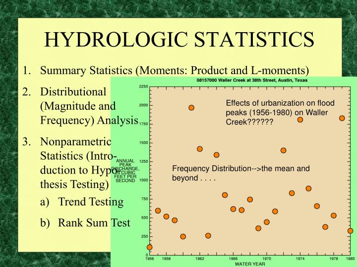
HYDROLOGIC STATISTICS. Summary Statistics (Moments: Product and L-moments) Distributional (Magnitude and Frequency) Analysis Nonparametric Statistics (Intro- duction to Hypo- thesis Testing) Trend Testing Rank Sum Test. Effects of urbanization on flood peaks (1956-1980) on Waller Creek??????.

E N D
HYDROLOGIC STATISTICS • Summary Statistics (Moments: Product and L-moments) • Distributional(Magnitude andFrequency) Analysis • NonparametricStatistics (Intro-duction to Hypo-thesis Testing) • Trend Testing • Rank Sum Test Effects of urbanization on flood peaks (1956-1980) on Waller Creek?????? Frequency Distribution-->the mean and beyond . . . .
Discrete and Continuous Random Variables Cumulative Distribution Function (cdf) expressed as functions have parameters Quantile Functions Statistical Expectation Quantiles median, quartiles, interquartile range plotting position estimators Plotting Positions1. order data x1≤x2≤ ...≤xn2. rank’em 1, 2, ..., n (i is rank)3. F(x) = i-0.40/n+0.2 Cunnane plotting-positions F(x) = i/n+1 Weibull plotting-positions PROBABILITY DISTRIBUTIONS
PLOTTING POSITIONS 1. order data x1≤x2≤ ...≤xn2. rank’em 1, 2, ..., n (i is rank) 3. F(x) = nonexceedance probability or just the percentile. 4. 1-F(x) = exceedance probability GENERAL FORMULA 1-F(x) = (i-a) / (n+1-2*a) Cunnane plotting-positions (a=0.40) F(x) = (i-0.40)/(n+0.2)“approx. quantile unbiased” Weibull plotting-positions (a=0) F(x) = i/(n+1)“unbiased [F(x)] for all distributions” Hazen plotting-positions (a=0.50) F(x) = (i-0.5)/n“long legacy” Blom plotting-positions (a=0.375) F(x) = (i-3/8)/(n+1/4) “optimal for normal distribution” MORE PLOTTING POSITION STUFF The true probability associated with the largest (and smallest) observation is a random variable with mean 1/(n+1) and a standard deviation of nearly 1/(n+1). Hence, all plotting position formula give crude estimates of the unknown probabilities associated with largest and smallest events. http://pubs.usgs.gov/twri/twri4a3/ See chapter 2
(Flow) Duration Curves--I • Simple, yet highly informative graphical summaries of the variability of a (daily) time series--Streamflow (flow-duration) • An FDC is a graph plotting the magnitude of a variable Q verses fraction of time the Q does not exceed a specified value [Q(F)]. The fraction of time can be thought of as probability and cumulative fraction of time is termed nonexceedance probability (F). • The probability refers to the frequency or probability of nonexceedance (or exceedance) in a “suitably long” period of time rather than probability of exceedance on a specific time interval (daily).
(Flow) Duration Curves--II • Area under the curve is equal to the average for the period. • Other statistics or statistical concepts visible include: median, quartiles, other percentiles, variability, and skewness. Steeper curves are associated with increasingly variable data. • The slopes and changes in the slope of the curves can be important diagnostics of streamflow conditions in a watershed.
(Flow) Duration Curves--III Duration curves for neighboring stations yield valuable insights into hydrologic or hydrogeologic processes
(Flow) Duration Curves--IV For natural streams Slope of FDC for upper end is determined by regional climate and characteristics of large precipitation events. Slope of the lower end is determined by geology, soils, topography. Slope of the upper end is relatively flat where snowmelt is the principal cause of floods and for large streams where floods are caused by long duration storms. Flashy watersheds and watersheds effected by short duration storms have steep upper ends. A flat lower end slope usually indicates that flows come from significant storage in ground water aquifers or frequency precipitation inputs.
SUMMARY STATISTICS Product Moments (PMs) L-moments—seen already, butwill study in detaillater in the semester. See powers--”product” Theoretical PMs----> E[ ] = Expectation operator In terms of PDF In terms of quantile function
SUMMARY STATISTICS Sample PMs----> Biased Estimators
SUMMARY STATISTICS Summary Statistics The uniformly minimum unbiased estimator of the standard deviation. PM Boundness!!!Careful in hydrologic data sets.
NONPARAMETRIC STATISTICS Nonparametric statistics (NP) are a branch of statistics based on the ranking or ranks of the data rather than the data values themselves. This fact has many desirable properties in hydrologic data analysis because data sets are often highly variable, measured with large error, censored, contaminated, and a host of other problems. • NP require fewer assumptions about the distribution generating the data. The normal or bell-shape curve assumption is NOT required. • NP are easier than classical statistics to apply. • NP are remarkably(?) straightforward to understand.
NONPARAMETRIC STATISTICS • NP can be used in situations that normal theory or classical statistics can not. • NP seem to sacrifice too much information. This is NOT the case. More often than not, NP are only slightly less efficient than classical statistics when distributions are normal. NP can be absurbly more efficient than classical statistics. • NP are robust in the presence of outliers, contaminated data, censored data, highly skewed data and so on. • Hollander, M., and Wolfe, D.A., 1973, Nonparametric statistical methods: John Wiley Inc., New York, 503 p.
NP STATISTICS—Trend Testing Trend Testing—that is the testing for temporal (time) trends—in data might be the most common use of NP in physical hydrology. Therefore, we’ll use trend testing as a starting point for introduction. Trend Testing = Relation Testing = Independence TestingKENDALL’S TAU
Kendall’s Tau—NP Trend Testing • We have n bivariate observations (X1,Y1), . . . , (Xn,Yn). • We want to test whether there is a relation between the X’s and the Y’s. We can not test for cause and effects—very important to remember. • We assume that each data pair are mutually independent and each pair is derived from the same population.
Kendall’s Tau—NP Trend Testing Define Kendall’s Tau byt = 2*Prob{(X1-X2)(Y1-Y2) > 0} - 1t = 0 if X’s and Y’s are unrelated because half of the time the X differences and Y differences would have the same sign. t = 2 * (1/2) - 1 = 0 -1 ≤t≤ 1 For each 1 ≤i < j≤ncalculate x(Xi,Xj,Yi,Yj) x(a,b,c,d) = score for . . . 1 if (a-b)(c-d) > 0 0 if (a-b)(c-d) = 0-1 if (a-b)(c-d) < 0
Kendall’s Tau—NP Trend Testing Sum up ones and minus ones and calculate the sum (K):K = S(i=1,n-1)S(j=i+1,n){x(a,b,c,d)}There are n*(n-1)/2 terms to compute. Compute t = 2K/[n*(n-1)], which is known as Kendall’s Rank Correlation Coefficient or simply “Kendall’s Tau”t estimates the probability parameter: Prob{(X1-X2)(Y1-Y2) > 0} = (t+1)/2t will generally be lower than values of the traditional correlation coefficient for linear associations of equal strength. “Strong” linear correlations of r > 0.9 correspond to t > 0.7. t measures all monotonic correlations (linear or nonlinear), and does not change with monotonic power transformations of X and/or Y [for example, log(X)].
INDEPENDENT DEPENDENT Kendall’s Tau—NP Trend Testing • Hypothesis Testing—We know that inherent randomness will produce a range of t differing from zero. If we know the distribution of t, hence K under conditions in which t = 0, we can perform a test by specifying some error or some tolerance in being right or wrong about whether the data is independent. Start with hypothesis, the Null Hypothesis, Ho, that the data is independent at the a level of significance, thena = a1 + a2 often it is taken that a1 = a2 reject Ho(t = 0) if K ≥ k(a2,n) or K ≤ -k(a1,n) accept Ha(t ≠ 0) if K < k(a2,n) or K > -k(a1,n) k is the null distribution of K, which we will investigate in more detail. We can also test whether t > 0, which means positive correlation between X and Y or whether t < 0 (negative correlation.)
Kendall’s Tau—NP Trend Testing t > 0 at the a significant level reject Ho(t = 0) if K ≥ k(a,n) accept Ha(t > 0) if K < k(a,n) t < 0 at the a significant level reject Ho(t = 0) if K ≤ -k(a,n) accept Ha(t < 0) if K > -k(a,n)
CIRCULAR STATISTICS Circular statistics are used to quantify the time of occurrence of hydrologic variables on a circle—typically on a yearly basis. • Successive samples of circular statistic results • The math :( • Really comprehensive analysis
Circular Statistics—see BOX 4-3 Circular statistics are used to quantify the time of occurrence of hydrologic variables on a circle—typically on a yearly basis. Two values require calculation: Average Time of Occurrence (Angle of the Mean) - analogous to the arithmetic mean Index of Seasonality - analogous to the standard deviation The average hydrologic quantity (say a monthly value) is considered to be a vector quantity. Length is proportional to the amount and direction (angle) of the time of the value.
Circular Statistics • Average Time of Occurrence (Angle of the Mean) • Time through the year (or other interval) is represented on a circle with (usually) each month assigned an angle. Think of the sin/cos terms as weight factors. • Resultant Angle Prime: fR’ = atan(S/C) • Resultant Angle (deal with quadrant):fR = fR’ if(S > 0 and C > 0)fR = fR’+180 if(C < 0)fR = fR’+360 if(S < 0 and C > 0) But other conversions are sometimes needed depending upon the output of the atan function.
Circular Statistics • Resultant Angle (deal with quadrant):$PHI = ( ($Sterm > 0 and $Cterm > 0) or • ($Sterm > 0 and $Cterm < 0) ) ? $PHIp : $PHIp+360;fR = fR’ fR = fR’+360 if[(S > 0 and C > 0) or (S < 0 and C < 0)] • 2. Index of Seasonality (IS) PR = sqrt(S2 + C2) IS = PR / (Total of Xm Values) In the Perl language
Circular Statistics List of examples of hydrologic variables on which circular statistics would be useful: Example: Total Rainfall = 36 inches-------------------------------------------------Season Rainfall sin cos-------------------------------------------------Spring (Mar.31;DoY=90) 4.00 0.9998 0.0215Summer(Jun.30;DoY=181) 16.00 .0258 -.9997Fall (Sept.30;DoY=273) 11.00 -.9999 -.0129Winter(Dec.31;DoY=365) 5.00 .0000 1.0000-------------------------------------------------S = -6.587; C = -11.05; f’=atan(S/C)=> 30.8 degreesf = 30.8 + 180 = 211 degreesPR = 12.87; IS = 12.87/36 = 0.357
Circular Statistics for 08155500 Barton Springs at Austin, Texas • 1978 to 2003 • Vector lengths are short • No definitive angle • Are these observations consistent with your expectation?
Circular Statistics for 08158000 Colorado River at Austin, Texas • 1899 to 2003 • Vector lengths are moderately long. • Concentration of angle near end of September to (through?) November. • Are these observations consistent with your expectation?
Circular Statistics for 08169000 Comal River at NewBraunfels, Texas • 1933 to 2002 • Vector lengths are short • No definitive angle--but perhaps more in January through March?
Circular Statistics for 08169000 Comal River at NewBraunfels, Texas
Circular Statistics for 08169000 Comal River at NewBraunfels, Texas