Download
1 / 1
10 likes | 80 Vues
Fall AGU 2006 Abstract # A31B-0875. A comparison of adjoint and analytical Bayesian inversion methods for constraining Asian sources of CO using satellite (MOPITT) measurements of CO columns

E N D
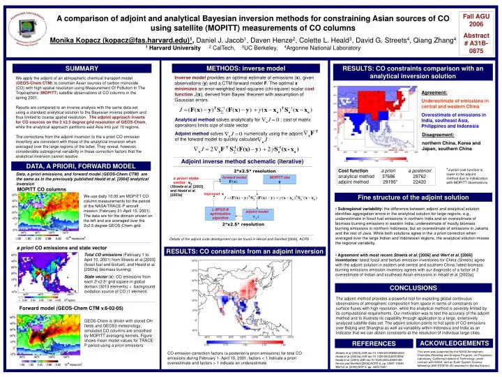
Fall AGU 2006 Abstract # A31B-0875 A comparison of adjoint and analytical Bayesian inversion methods for constraining Asian sources of CO using satellite (MOPITT) measurements of CO columns Monika Kopacz (kopacz@fas.harvard.edu)1, Daniel J. Jacob1, Daven Henze2, Colette L. Heald3, David G. Streets4, Qiang Zhang4 1 Harvard University2 CalTech, 3UC Berkeley, 4Argonne National Laboratory METHODS: inverse model RESULTS: CO constraints comparison with an analytical inversion solution SUMMARY Inverse modelprovides an optimal estimate of emissions (x), given observations (y) and a CTM forward model F. The optimal xminimizes an error-weighted least-squares (chi-square) scalar cost functionJ(x), derived from Bayes’ theorem with assumption of Gaussian errors. We apply the adjoint of an atmospheric chemical transport model (GEOS-Chem CTM) to constrain Asian sources of carbon monoxide (CO) with high spatial resolution using Measurement Of Pollution In The Troposphere (MOPITT) satellite observations of CO columns in the spring 2001. Results are compared to an inverse analysis with the same data set using a standard analytical solution to the Bayesian inverse problem and thus limited to coarse spatial resolution. The adjoint approach inverts for CO sources on the 2 x2.5 degree grid resolution of GEOS-Chem, while the analytical approach partitions east Asia into just 10 regions. The corrections from the adjoint inversion to the a priori CO emission inventory are consistent with those of the analytical inversion when averaged over the large regions of the latter. They reveal, however, considerable subregional variability in these correction factors that the analytical inversion cannot resolve. Agreement: Underestimate of emissions in central and western China Overestimate of emissions in India, southeast Asia, Philippines and Indonesia Analytical method solves analytically for ; cost of matrix operations limits size of state vector Adjoint methodsolves numerically using the adjoint of the forward model to quickly calculate : Disagreement: northern China, Korea and Japan, southern China Adjoint inverse method schematic (iterative) DATA, A PRIORI, FORWARD MODEL *a priori cost function is lower in the adjoint method due to initialization with MOPITT observations Cost function a priori a posteriori analytical method 37686 28762 adjoint method 29195* 22420 2°x2.5° resolution Data, a priori emissions, and forward model (GEOS-Chem CTM) are the same as in the previously published Heald et al. [2004] analytical inversion MOPITT obs y forward model a priori state vector xa (Streets et al. [2003] and Heald et al. [2003a] MOPITT CO columns improvedx Fine structure of the adjoint solution We use daily 10:30 am MOPITT CO column measurements for the period of the NASA/TRACE-P aircraft mission (February 21-April 10, 2001). The data are for the domain shown on the left and are averaged over the 2x2.5 degree GEOS-Chem grid (c) (b) (a) • Subregional variability: the difference between adjoint and analytical solution identifies aggregation errors in the analytical solution for large regions, e.g., underestimate in fossil fuel emissions in northern India and an overestimate of biomass burning emissions in eastern India; underestimate of mostly biomass burning emissions in northern Indonesia, but an overestimate of emissions in Jakarta and the rest of Java. While both solutions agree in the a priori correction when averaged over the large Indian and Indonesian regions, the analytical solution misses the regional variability. • Agreement with most recent Streets et al. [2006] and Werf et al. [2006] inventories: latest fossil and biofuel emission inventories for China (Streets) agree with the adjoint solution in eastern and central and southern China; latest biomass burning emissions emission inventory agrees with our diagnostic of a factor of 2 overestimate of Indian and southeast Asian emissions in Heald et al. [2003a]. L-BFGS-B optimization algorithm adjoint model 2°x2.5° resolution Details of the adjoint code development can be found in Henze and Seinfeld [2006], ACPD a priori CO emissions and state vector RESULTS: CO constraints from an adjoint inversion Total CO emissions (February 1 to April 10, 2001) from Streets et al.[2003] (fossil fuel and biofuel); and Heald et al. [2003a] (biomass burning) State vector (x): CO emissions from each 2ox2.5o grid square in global domain (3013 elements) + background oxidation source of CO (1 element) CONCLUSIONS The adjoint method provides a powerful tool for exploiting global continuous observations of atmospheric composition from space in terms of constraints on surface fluxes with high resolution, while the analytical method is severely limited by its computational requirements. Our motivation was to test the accuracy of the adjoint method and to illustrate its capability through application to a large, extensively analyzed satellite data set. The adjoint solution points to hot spots of CO emissions over Beijing and Shanghai as well as variability within Indonesia and India as an indicator that we can obtain constraints at the resolution of individual large cities. Forward model (GEOS-Chem CTM v.6-02-05) GEOS-Chem is driven with stored OH fields and GEOS3 meteorology; simulated CO columns are smoothed by MOPITT averaging kernels. Figure shows mean model values for TRACE-P period using a priori emissions ACKOWLEDGEMENTS REFERENCES This work was supported by the NASA Atmospheric Chemistry Modeling and Analysis Program; Jet Propulsion Laboratory, California Institute of Technology, under contract with NASA, and an Earth System Science fellowship (#06-ESSF06-45) awarded to Monika Kopacz. CO emission correction factors (a posteriori/a priori emissions) for total CO emissions during February 1- April 10, 2001; factors < 1 indicate a priori overestimate and factors > 1 indicate an underestimate Streets et al. [2003] JGR doi:10.1029/2003GB002040 Heald et al. [2003a] JGR doi:10.1029/2002JD003082 Heald et al. [2004] JGR doi:10.1029/2004JD005185 Henze and Seinfeld [2006] ACPD 6, pp.10591-10648 Werf et al. [2006] ACP 6, pp. 3423-3441