Download
1 / 26
260 likes | 420 Vues
Simulated Inductance. Experiment 25. Modification from Lab Manual. Write a MatLAB program Determine the transfer function Calculate the output voltage in phasor notation at the corner frequency. obtain a Bode plot Plot of AC Sweep in PSpice simulation y-axis should be in dB

E N D
Simulated Inductance Experiment 25
Modification from Lab Manual • Write a MatLAB program • Determine the transfer function • Calculate the output voltage in phasor notation at the corner frequency. • obtain a Bode plot • Plot of AC Sweep in PSpice simulation • y-axis should be in dB • Frequency range from 1 kHz to 10 MHz • Construct a gyrator that has an effective inductance of 10mH. • Compare the operation of the gyrator with the 10mH inductor in an RL circuit where R = 2 kW.
Gyrator • Inductors are far from ideal devices • Parasitic resistance because of the length of wire used to form the inductor. • Parasitic capacitance because of coupling between parallel loops of wire.
Integrated Circuits • Inductors are three dimensional devices, usually free standing • Very difficult to fabricate using standard semiconducting processes and to integrate in a silicon wafer.
Gyrator • Operational Amplifier circuit that has a frequency response similar to an inductor.
Low Pass RL Filter At 0Hz, Vout = Vin. As the frequency increases and the inductor begins to act like an open, Vout approaches 0V.
High Pass RL Circuit At 0Hz, Vout = 0V. As the frequency increases and the inductor begins to act like an open, Vout approaches Vin.
Information from 741 Datasheet Operational Amplifiers are designed to have large open loop gain. But, the frequency response of the circuit has been sacrificed to achieve this.
Applications for Gyrator • Low frequency (f < 500 kHz) applications in: • Audio Engineering • Biomedical Engineering • Certain areas of power electronics
Defining a Vector Three elements t=[0,.1,3] or t=[0 .1 3] t = 0 0.1000 3.0000 Four Elements t=[0:3] t = 0 1 2 3 Elements that include 0, then 0.1, and then increments of 1 until it reaches the largest number ≤ 3 t=[0,.1:3] t = 0 0.1000 1.1000 2.1000 Thirty one elements between 0 and 3 in increments of 0.1 t=[0:.1:3] t = 0 0.1000 0.2000 0.3000 0.4000 0.5000 0.6000 0.7000 0.8000 0.9000 1.0000 1.1000 1.2000 1.3000 1.4000 1.5000 1.6000 1.7000 1.8000 1.9000 2.0000 2.1000 2.2000 2.3000 2.4000 2.5000 2.6000 2.7000 2.8000 2.9000 3.0000
MatLAB Suppose you have determined that the transfer function for your filter is: • You can put this transfer function into MatLAB • Define two vectors • A = [An, An-1, ….., A1, A0] where n, m ≥ 0 and • B = [Bm, Bm-1, ….., B1, B0] n does not have to equal m • H = tf(A,B)
Example High pass filter with a single-pole/single-zero • Let RC = 104 s/rad • A = [0, 10e3] • B = [1 10e3] • H = tf(A,B) 10000s H = --------- is returned when you run the program 10000s + 1
MatLAB: Bode Plots • Once you have entered the transfer function into MatLAB, you can use a predefined function ‘bode’ to automatically generate plots of the magnitude and phase vs. frequency. Enter: bode(H)
Complex Numbers • The default symbol for √-1 is i. However, MatLAB does recognize that j is equivalent to i. • The coefficient of the imaginary number must be placed before the ‘i’ or ‘j’. • If you typed c = 2-3j, MatLAB interprets it as c = 2.0000 - 3.0000i • To find components of complex number • real(c) returns 2 • imag(c) returns -3
Magnitude and Phase • Magnitude of a complex number • Is the square root of the square of the real component plus the square of the imaginary component • Phase of a complex number • Is the arc tangent of the imaginary component divided by the real component • Must change to degrees if the output of the arc tangent is given in radians