Download
1 / 69
710 likes | 850 Vues
Electromagnetic multipole moments of baryons. Alfons Buchmann University of Tübingen. Introduction Method Observables Results Summary. NSTAR 2007, Bonn, 5-8 September 2007. 1. Introduction. What can we learn from electromagnetic multipole moments?.

E N D
Electromagnetic multipole moments of baryons Alfons Buchmann University of Tübingen • Introduction • Method • Observables • Results • Summary NSTAR 2007, Bonn, 5-8 September 2007
What can we learn from electromagnetic multipole moments? Electromagnetic multipole moments of baryons are interesting observables. • They are directly connected with spatial distributions of • charges and currents inside baryons. • They provide fundamental information on baryonic • structure, • size, • shape .
Example: Proton magnetic moment Experimental discovery by Frisch and Stern in 1933 p (exp) 2.5 N p is very different from value predicted by Dirac equation p (Dirac)= 1.0 N Conclusion: proton has an internal structure. Measurement of proton charge radius by Hofstadter et al. in 1956 r²p(exp) (0.81 fm)²
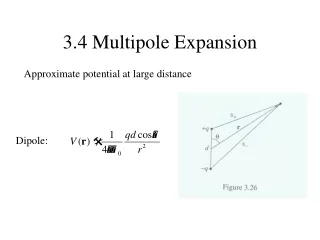
–q +q +q –q +q –q +q +q +q –q + + + –q –q –q +q +q ~ q0 + d1 + Q2 +3 + monopole octupole quadrupole dipole Multipole expansion of charge distribution for a system of point charges J=0 J=1 J=2 J=3
charge monopole C0 magnetic dipole M1 Example: N(939) Ji=1/2 • Advantage of multipole expansion • multipole operators MJtransfer definite angular momentum and parity • angular momentum and parity selection rules apply, • e.g. only even charge multipoles • few multipoles suffice to describe charge and current density Baryon B with total angular momentum Ji 2 Ji+ 1 electromagnetic multipoles
Blanpied et al., PRC 64 (2001) 025203 Tiator et al., EPJ A17 (2003) 357 Buchmann et al., PRC 55 (1997) 448 Example: N quadrupole moment Recent electron-proton scattering experiments provide evidence for a nonzero p +(1232) transition quadrupole moment data theory neutron charge radius
Definition of intrinsic quadrupole moment prolate oblate What can be learned from these results? • both N and have nonspherical chargedistributions • to learn more about the geometric shape of both systems, • one has to calculate their intrinsic quadrupole moments Q0 concentrated along z-axis 3z²- term dominates Q0 > 0 concentrated in equatorial plane r² -term dominates Q0 < 0
lab frame body-fixed frame Intrinsic (Q0) vs. spectroscopic (Q) quadrupole moment J=1/2 Q=0 even if Q0 0. projection factor
Buchmann and Henley (PRC 63 (2001) 015202) have calculated Q0 in three nucleon models. All models agree as to the sign of Q0. For example, in the quark model they find Q0 (N) = -rn2 > 0 Q0 () = rn2 < 0. Neutron charge radius determines sign and size of N and intrinsic quadrupole moments.
Interpretation in pion cloud model Q0 > 0 Q0 < 0 prolate oblate A. J. Buchmann and E. M. Henley, Phys. Rev. C63, 015202 (2001)
Summary In the last decade interesting experimental and theoretical results on the charge quadrupolestructure of the N and system have been obtained. Based on model calculations of the intrinsic quadrupole moments of both systems, it has been proposed that the charge distributions of N(939) and (1232) possess considerable prolate and oblate deformations. Review: V. Pascalutsa, M. Vanderhaeghen, S.N. Yang, Phys. Rep. 437, 125 (2007)
What about higher multipole moments? Presently, practically nothing is known about magnetic octupole moments of decuplet baryons. Information needed to reveal structural details of spatial current distributions in baryons.
General parametrization method Basic idea 1) Define for observable at hand a QCD operator Ô and QCD eigenstates B 2) Rewrite QCD matrix element <B|Ô|B in terms of spin-flavor space matrix elements including all spin-flavor operators allowed by Lorentz and inner QCD symmetries (G. Morpurgo, 1989)
... auxilliary 3 quark QCD state ... exact QCD state containing q, (qq), (qq)2, g, ... ... unitary operator dresses auxilliary state with quark-antiquark pairs and gluons ... spin-flavorstate ... spin-flavor operator V ...unitary operator B ...auxilliary 3q states QCD matrix element spin-flavor matrix element
one-body two-body three-body General spin-flavor operator O constants A, B, and C parametrize orbital and color matrix elements. These are determined from experiment. O[i] all allowed invariants in spin-flavor space Which spin-flavor operators are allowed? Operator structures determined from symmetry principles.
Strong interaction symmetries Strong interactions are approximately invariant under SU(3) flavor and SU(6) spin-flavor symmetry transformations.
S n p D- D0 D+ D++ S*+ S*- S*0 S+ S0 S- L0 X*- X*0 X- X0 W SU(3) flavor multiplets 0 -1 -2 octet decuplet -3 J=3/2 J=1/2 T3 -1 -1/2 0 +1/2 +1 -3/2 -1/2 +1/2 +3/2
SU(6) spin-flavor symmetry ties together SU(3) multiplets with different spin and flavor into SU(6) spin-flavor supermultiplets
S T3 SU(6) spin-flavor supermultiplet ground state baryon supermultiplet
SU(6) spin-flavor is a symmetry of QCD SU(6) symmetry is exact in the large NC limit of QCD. For finite NC,the symmetry is broken. The symmetry breaking operators can be classified according to powers of 1/NC attached to them. This leads to a hierarchy in importance of one-, two-, and three-quark operators, i.e., higher order symmetry breaking operators are suppressed by higher powers of 1/NC.
strong coupling two-body three-body 1/NC expansion of QCD processes
SU(6) spin-flavor symmetry breaking by spin-flavor dependent two- and three-quark operators σk m k These lift the degeneracy between octet and decuplet baryons.
two-body three-body Example: quadrupole moment operator no one-quark contribution
ek ei g g 2-quark current 3-quark current SU(6) spin-flavor symmetry breaking by spin-flavor dependent two- and three-quark operators e.g. electromagnetic current operator ei ... quark charge si ... quark spin mi ... quark mass
Origin of these operator structures 1-quark operator 2-quark operators (exchange currents)
Summary Parametrization method • based on symmetries of QCD • quark-gluon dynamics reflected in 1/Nc hierarchy • employs complete operator basis in SU(6) spin-flavor space
Magnetic octupole moments of decuplet baryons Decuplet baryons have Ji=3/2 4 electromagnetic multipoles charge monopole moment q+=1 charge quadrupole moment Q+ rn2 magnetic dipole moment +p magnetic octupole moment + = ? Example: +(1232)
Definition of magnetic multipole operator special cases: J=1 J=3
replace magnetic moment density by charge density Magnetic octupole moment analogous to charge quadrupole moment Q
Magnetic octupole moment measures the deviation of the magnetic moment distribution from spherical symmetry > 0 magnetic moment density is prolate < 0 magnetic moment density is oblate
Construction of octupole moment operator in spin-flavor space • ~ MJ=3 ... tensor of rank 3 rank 3 tensor built from quark spin operators 1 • ~ i1 j1 k1 • • involves Pauli spin matrices of three different quarks is a three-quark operator
If two Pauli spin operators in had the same particle index e.g. i=j=1 reduction to a single spin matrix due to the SU(2) spin commutation relations is neccessarily a three-quark operator
Allowed spin-flavor operators ei...quark charge i...quark spin two-quark quadrupole operator multiplied by spin of third quark three-quark quadrupole operator multiplied by spin of third quark Do we need both?
0-body 1-body 2-body 3-body Spin-flavor selection rules M 0 only if R transforms according to representations found in the product
There is a unique three-quark operator transforming according to 2695 dim. rep. of SU(6). We can take either one of the two spin-flavor structures. Explicit calculation of both operators give the same results for decuplet baryons.
Matrix elements qB baryon charge In the flavor symmetry limit, magnetic octupole moments of decuplet baryons are proportional to the baryon charge
Introduce SU(3) symmetry breaking SU(3) symmetry breaking parameter flavor symmetry limit r=1
Efficient parametrization of baryon octupole moments in terms of just one constant C.
Relations among octupole moments There are 10 diagonal octupole moments. These are expressed in terms of 1 constant C. There must be 9 relations between them.
Diagonal octupole moment relations These 6 relations hold irrespective of how badly SU(3) is broken.
3 r-dependent relations Typical size of SU(3) symmetry breaking parameter r=mu/md=0.6
Information on the geometric shape of current distribution in baryons from sign and magnitude of .
Numerical results Determine sign and magnitude of using various approaches 1) pion cloud model 2) experimental N N*(1680) transition octupole moment 3) current algebra approach
0 Y01 Estimate of in pion cloud model spherical core surrounded by P-wave cloud ´ cloud bare core