Download

1 / 37
380 likes | 733 Vues
THE MULTIPLIER MODEL. Chapter 26. Today’s lecture will:. Explain the difference between induced and autonomous expenditures. Demonstrate how the level of income is graphically determined in the multiplier model. Use the multiplier equation to determine equilibrium income.

E N D
THE MULTIPLIER MODEL Chapter 26
Today’s lecture will: • Explain the difference between induced and autonomous expenditures. • Demonstrate how the level of income is graphically determined in the multiplier model. • Use the multiplier equation to determine equilibrium income.
Today’s lecture will: • Explain how the multiplier process amplifies shifts in autonomous expenditures. • Demonstrate how fiscal policy can eliminate recessionary and inflationary gaps. • Discuss six reasons why the multiplier model might be misleading.
The Multiplier Model • The multiplier model explains how an initial change in expenditures changes equilibrium output when the price level is fixed. • An initial expenditure causes additional induced (multiplier) effects. • The multiplier model quantifies the effect of changes in aggregate expenditures on aggregate output.
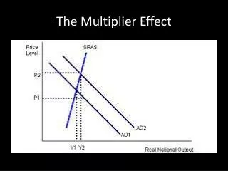
Price level Induced shift (Multiplier effects) Initial shift ? Cumulative shift Real output The AS/AD Model When Prices are Fixed 20 P0 Short-run aggregate supply AD1 AD0
B C A Potential income 45º The Aggregate Production Curve Real production • Aggregate production – the total amount of goods and services produced in an economy. • Production creates an equal amount of income, so the 45° line represents production=income. Aggregate production (production = income) $4,000 0 $4,000 Real income
Aggregate Expenditures • Aggregate expenditures – the total amount of spending on final goods and services: • Consumption – spending by consumers • Investment – spending by businesses • Government spending • Net foreign spending – U.S. exports minus U.S. imports
Autonomous and Induced Expenditures • Autonomous expenditures – expenditures that do not systematically vary with income. • They remain constant at all levels of income. • Induced expenditures – expenditures that change as income changes. • When income changes, they change by less than income.
The Marginal Propensity to Expend • Marginal propensity to expend (mpe) – the ratio of the change in aggregate expenditures to a change in income. • The mpe is an aggregation of the change in each of the components of aggregate expenditures to changes in income. • The mpe, always between 0 and 1, is the slope of the aggregate expenditures curve.
Aggregate Expenditures Curve Aggregate Expenditures $6500 $6000 $5500 Real Expenditures Induced Expenditures $3000 Autonomous Expenditures $5000 $7000 $6000 Real Income
Components of the MPE • Marginal propensity to consume (mpc) – the change in consumption that occurs with a change in income. • The mpc is less than one because individuals save a portion of an increase in income. • Marginal propensity to import – the change in imports that occurs with a change in income. • Income taxes reduce people’s income which lowers their expenditures.
The Aggregate Expenditures Function • The relationship between aggregate expenditures and income can be expressed mathematically as: AE = AE0 + mpeY AE0 = C0 + I0 + G0 + (X0 – M0) induced autonomous
Graphing the Expenditures Function Autonomous consumption is 100 Autonomous investment is 40 Autonomous government spending is 20 Autonomous net exports is 30 Marginal propensity to expend is 0.6 AE 310 Slope = 0.6 190 200 400 600 Real income
Shifts in the Expenditures Function • The aggregate expenditures curve shifts when autonomous C, I, G, or (X-M) change. • The multiplier model is an historical model most useful for analyzing shifts in autonomous expenditures. • Shifts in aggregate expenditures lead to a change in income from its current level.
Equilibrium Aggregate Income AE Aggregate production Aggregate expenditures 14,000 • At equilibrium, AE ($10,000) = production or Y ($10,000). • At Y = $14,000, AE<Y, so inventories increase by $2000. • At Y = $4000, AE>Y, so inventories fall below desired levels by $3000. 12,000 10,000 AE = 5,000 + 0.5Y Equilibrium 7,000 5,000 AE0 = 5,000 4,000 10,000 14,000 Real income (in dollars)
The Multiplier Equation • The multiplier equation can be used to find equilibrium income. • The expenditures multiplier reveals how much income will change in response to a change in autonomous expenditures. • As the mpe increases, the multiplier increases. Y = multiplier x autonomous expenditures
The Multiplier Process AP $7,000 • At incomelevels A and B, the economy is not in equilibrium. • If the economy is at A, output > aggregate expenditures by $1500. • Businesses decrease production, which decreases income and expenditures until production and expenditures are equal at C. A1 AE 5,500 A2 4,750 4,000 Real expenditures 2,500 B1 2,000 B2 $1,000 B $4,000 C $7,000 A Real income (in dollars)
The Circular Flow and the Multiplier Process • The circular flow model illustrates the multiplier process. • The flow of expenditures equals the flow of income. • Theflow of income spent on imports is a leakage from the circular flow. • Autonomous expenditures are injections into the circular flow. Aggregate income Firms Households Aggregate expenditures
The Multiplier Model in Action • The multiplier model illustrates how a change in autonomous expenditures changes the equilibrium level of income. • When autonomous expenditures shift, the multiplier process is called into play. • Any initial shock (a change in autonomous AE) is multiplied in the adjustment process.
Shifts in the AE Curve C, I E1 AE1 = 250 + .5Y E1 ΔAEA=100 Δ 500 100 A AE2 = 150 + .5Y B 100 ΔAEB=50 E2 300 C C C 50 100 250 25 150 E2 25 $200 0 $300 $500 200 Real income
mpe = .5 mpe = .8 100 100 80 64 51.2 50 40.96 25 6.25 12.5 Multiplier = 1/(1-0.5) = 2 Multiplier = 1/(1-0.8) = 5 The First Steps of Two Multipliers
Reasons for Shifts in Aggregate Expenditures • Natural disasters • Changes in investment caused by technological developments • Shifts in government expenditures • Large changes in the exchange rate • Changes in consumer sentiment
4,090 $4,090 An Increase in Autonomous Expenditures Real expenditures Aggregate production AE1 $4,210 30 AE0 1,052.5 30 1,022.5 $120 0 $4,210 Real income
Real World Examples of Shifts in Aggregate Expenditures • The U.S. economy boomed from 1998-2001 and fell into a recession after September, 2001. • Consumer confidence increased autonomous consumption through mid-2001. • Consumer spending and investment fell after the terrorist attacks in September 2001.
Real World Examples of Shifts in Aggregate Expenditures • Aggregate income and production fell in Japan during the 1990s. • A dramatic appreciation of the yen decreased Japanese exports. • Autonomous consumption fell as consumer confidence decreased. • Suppliers responded by laying off workers and cutting production.
Fiscal Policy and the Multiplier • Expansionary policy is appropriate when there is a recessionary gap. • The increased spending leads to a multiple increase in AE, thereby closing the gap. • Contractionary policy is appropriate when there is an inflationary gap. • The decreased spending leads to a multiple decrease in AE, thereby closing the gap.
Expansionary Fiscal Policy Aggregate production Potential output LAS Initial expenditures increase AE1 AE0 Multiplier effect E2 $120 ∆G = $60 $60 mpe = 0.67 SAS P0 AE1 = 333 + 0.67Y E1 AD0 AD1΄ Recessionary gap $180 AD1 $1,000 $1,180 Real income $1,000 $1,180 Real income
Contractionary Fiscal Policy Aggregate production Potential output LAS AE0 AE1 P2 B E1 ∆G = $200 $1,000 A mpe = 0.8 SAS P1 AE1 = 800 + 0.8Y AD0 E2 Inflationary gap AD1 $4,000 $5,000 Real income $4,000 $5,000 Real income
Limitations of the Multiplier Model • The multiplier model is not a complete model. • The multiplier model does not determine equilibrium income from scratch. • It can only estimate the direction and rough sizes of autonomous demand shifts. • Shifts in aggregate expenditures that occur in response to autonomous expenditures may be overstated.
Limitations of the Multiplier Model • The price level will often change in response to changes in aggregate demand, but the multiplier model assumes that the price level is fixed. • Forward-looking expectations complicate the adjustment process. • Most people act upon their expectations of the future. • Rational expectations model – all decisions are based upon the expected equilibrium in the economy.
Limitations of the Multiplier Model • Shifts in expenditures may reflect desired changes in supply and demand, rather than simply suppliers responding to changes in demand. • Real business cycle theory – fluctuations in the economy reflect real phenomena such as simultaneous shifts in supply and demand, not simply supply responses to demand shifts.
Limitations of the Multiplier Model • Expenditures depend on much more than current income. • Permanent income hypothesis – expenditures are determined by permanent or lifetime income. • The mpc out of current income could be zero, which would make the multiplier equal to one.
Summary • The multiplier model focuses on the induced effect that a change in production has on expenditures, which affects production, and so on. • In equilibrium in the multiplier model, aggregate production (income) must equal planned aggregate expenditures (AE). • AE = C + I + G + (X – M) • The mpe tells us the change in expenditures that occurs with a change in income.
Summary • Equilibrium can be calculated using the multiplier equation: Y = multiplier x autonomous expenditures • The multiplier tells us how much a change in autonomous expenditures will change equilibrium income. • The multiplier equals 1(1-mpe).
Summary • Expansionary fiscal policy, increasing government expenditures or decreasing taxes, is represented as an upward shift of the AE curve or a rightward shift in the AD curve. • Contractionary fiscal policy, decreasing government spending or increasing taxes, is represented as a downward shift of the AE curve or a leftward shift of the AD curve.
Summary • The multiplier model has limitations: • It is incomplete without information about where the economy started and what is the desired level of output. • It overemphasizes shifts in AE. • It assumes that the price level is fixed. • It doesn’t take expectations into account. • It ignores the possibility that shifts in expenditures are desired. • It ignores the possibility that consumption is based on lifetime income, not current income.
Assume that the mpe is 0.75 and autonomous expenditures are $1000. Review Question 26-1 What is the aggregate expenditures function? • AE = 1000 + .75Y Review Question 26-2 What is equilibrium income? • Y = AE at equilibrium, so: • Y = 1000 + .75Y • .25Y = 1000 • Y = $4000 Review Question 26-3 What happens if income is $4800? • AE = 1000 + .75(4800) = $4600 • If income is $4800, inventories of $200 accumulate causing output and income to decrease until output and income equal aggregate expenditures at $4000.