Download
1 / 17
180 likes | 409 Vues
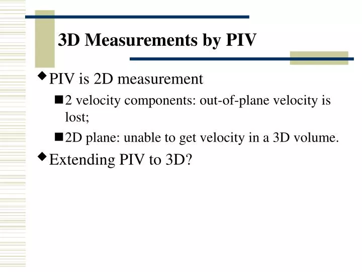
3D Measurements by PIV. PIV is 2D measurement 2 velocity components: out-of-plane velocity is lost; 2D plane: unable to get velocity in a 3D volume. Extending PIV to 3D?. Technique. Dimension of velocity field. Dimension of observation volume. Remark. Stereoscopic PIV. 3D. 2D.

E N D
3D Measurements by PIV • PIV is 2D measurement • 2 velocity components: out-of-plane velocity is lost; • 2D plane: unable to get velocity in a 3D volume. • Extending PIV to 3D?
Technique Dimension of velocity field Dimension of observation volume Remark Stereoscopic PIV 3D 2D Recover out-of-plane velocity Dual plane PIV 3D Scanning PIV 3D Time delayed measurement 3D PTV Seldom used due to low resolution Holographic PIV True volumetric measurement with high ressolution Extension of PIV technique
Camera 3D Scanning PIV Drum scanner • Scanning a volume to get the depth information • Multiple frames recording and high-speed scanner are required • Time lag between frames: quasi-3D measurement Scanning volume Laser
3D Particle Tracking Velocimetry (PTV) • Extracting 2D particle locations from images captured from different views; • Reconstructing 3D particle locations according to the parameters of cameras and calibration information; • Tracking 3D particles in the volume to get the velocity • Extremely low resolution (hundreds of velocity map in one volume): cannot overlap
Fundamentals of stereo vision True 3D displacement (DX,DY,DZ) is estimated from a pair of 2D dis- placements (Dx,Dy) as seen from left and right camera respectively
Camera Camera Camera Camera Types of Stereo recording geometry Angular arrangement: Different parts of the plane cannot be all in focus Parallel arrangement: Share only partial field of view
The proper stereo recording geometry Properly focusing the entire field of view with an off-axis camera requires tilting of the camera back-plane to meet the Scheimpflug condition — The image, lens and object planes must cross each other along a common line in space
Mapping from 2D image back to 3D 3D evaluation requires a numerical model, describing how objects in 3D space are mapped onto the 2D image plane of each of the cameras - The pinhole camera model is based on geometrical optics, and leads to the so-called direct linear transformation (DLT) - With the DLT model, coefficients of the A-matrix can in principle be calculated from known angles, distances and so on for each camera. - In practice not very accurate, since, as any experimentalist will know, once you are in the laboratory you cannot set up the experiment exactly as planned, and it is very difficult if not impossible to measure the relevant angles and distances with sufficient accuracy. Hence, parameters for the numerical model are determined through camera calibration
Camera calibration Images of a calibration target are recorded. The target contains calibration markers (dots), true (x,y,z) positions are known. Comparing known marker positions with corresponding marker positions on each camera image, model parameters are adjusted to give the best possible fit.
Overlapping fields of view 3D evaluation is possible only within the area covered by both cameras. Due to perspective distortion each camera covers a trapezoidal region of the light sheet. Careful alignment is required to maximize the overlap area. Interrogation grid is chosen to match the spatial resolution.
Left / Right 2D vector maps Left & Right camera images are recorded simultaneously. Conventional PIV processing produce 2D vector maps representing the flow field as seen from left & right. Using the camera model including parameters from the calibration, the points in the chosen interrogation grid are now mapped from the light sheet plane onto the left and right image plane (CCD-chip) respectively. The vector maps are re-sampled in points corresponding to the interrogation grid. Combining left / right results, 3D velocities are estimated.
Overlap area withinterrogation grid Resulting 3D vector map Left 2D vector map Right 2D vector map 3D reconstruction
Dantec 3D-PIV system components • Seeding • PIV-Laser(Double-cavity Nd:Yag) • Light guiding arm &Lightsheet optics • 2 cameras on stereo mounts • FlowMap PIV-processor with two camera input • Calibration target on a traverse • FlowManager PIV software • FlowManager 3D-PIV option
Recipe for a 3D-PIV experiment • Record calibration images in the desired measuring position(Target and traverse defines the co-ordinate system!) • Align the lightsheet with the calibration target • Record calibration images using both cameras • Record simultaneous 2D-PIV vector maps using both cameras • Calibration images and vector maps is read into FlowManager • Perform camera calibration based on the calibration images • Calculate 3D vectors based on the two 2D PIV vector maps and the camera calibration