Download
1 / 17
180 likes | 376 Vues
Multiple Linear Regression. Response Variable: Y Explanatory Variables: X 1 ,..., X k Model (Extension of Simple Regression): E ( Y ) = a + b 1 X 1 + + b k X k V ( Y ) = s 2

E N D
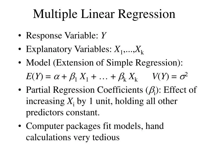
Multiple Linear Regression • Response Variable: Y • Explanatory Variables: X1,...,Xk • Model (Extension of Simple Regression): • E(Y) = a + b1X1 + + bkXkV(Y) = s2 • Partial Regression Coefficients (bi): Effect of increasing Xi by 1 unit, holding all other predictors constant. • Computer packages fit models, hand calculations very tedious
Prediction Equation & Residuals • Model Parameters: a, b1,…, bk, s • Estimators: a, b1, …, bk, • Least squares prediction equation: • Residuals: • Error Sum of Squares: • Estimated conditional standard deviation:
Commonly Used Plots • Scatterplot: Bivariate plot of pairs of variables. Do not adjust for other variables. Some software packages plot a matrix of plots • Conditional Plot (Coplot): Plot of Y versus a predictor variable, seperately for certain ranges of a second predictor variable. Can show whether a relationship between Y and X1 is the same across levels of X2 • Partial Regression (Added-Variable) Plot: Plots residuals from regression models to determine association between Y and X2, after removing effect of X1 (residuals from (Y , X1) vs (X2 , X1))
Example - Airfares 2002Q4 • Response Variable: Average Fare (Y, in $) • Explanatory Variables: • Distance (X1, in miles) • Average weekly passengers (X2) • Data: 1000 city pairs for 4th Quarter 2002 • Source: U.S. DOT
Example - Airfares 2002Q4 Scatterplot Matrix of Average Fare, Distance, and Average Passengers (produced by STATA):
Example - Airfares 2002Q4 Partial Regression Plots: Showing whether a new predictor is associated with Y, after removing effects of other predictor(s): After controlling for AVEPASS, DISTANCE is linearly related to FARE After controlling for DISTANCE, AVEPASS not related to FARE
Standard Regression Output • Analysis of Variance: • Regression sum of Squares: • Error Sum of Squares: • Total Sum of Squares: • Coefficient of Correlation/Determination: R2=SSR/TSS • Least Squares Estimates • Regression Coefficients • Estimated Standard Errors • t-statistics • P-values (Significance levels for 2-sided tests)
Multicollinearity • Many social research studies have large numbers of predictor variables • Problems arise when the various predictors are highly related among themselves (collinear) • Estimated regression coefficients can change dramatically, depending on whether or not other predictor(s) are included in model. • Standard errors of regression coefficients can increase, causing non-significant t-tests and wide confidence intervals • Variables are explaining the same variation in Y
Testing for the Overall Model - F-test • Tests whether any of the explanatory variables are associated with the response • H0: b1==bk=0 (None of Xs associated with Y) • HA: Not all bi = 0 The P-value is based on the F-distribution with k numerator and (n-(k+1)) denominator degrees of freedom
Testing Individual Partial Coefficients - t-tests • Wish to determine whether the response is associated with a single explanatory variable, after controlling for the others • H0: bi = 0 HA: bi 0 (2-sided alternative)
Modeling Interactions • Statistical Interaction: When the effect of one predictor (on the response) depends on the level of other predictors. • Can be modeled (and thus tested) with cross-product terms (case of 2 predictors): • E(Y) = a + b1X1 + b2X2 + b3X1X2 • X2=0 E(Y) = a + b1X1 • X2=10 E(Y) = a + b1X1 + 10b2 + 10b3X1 • = (a + 10b2) + (b1 + 10b3)X1 • The effect of increasing X1 by 1 on E(Y) depends on level of X2, unless b3=0 (t-test)
Comparing Regression Models • Conflicting Goals: Explaining variation in Y while keeping model as simple as possible (parsimony) • We can test whether a subset of k-g predictors (including possibly cross-product terms) can be dropped from a model that contains the remaining g predictors. H0: bg+1=…=bk =0 • Complete Model: Contains all k predictors • Reduced Model: Eliminates the predictors from H0 • Fit both models, obtaining the Error sum of squares for each (or R2 from each)
Comparing Regression Models • H0: bg+1=…=bk = 0 (After removing the effects of X1,…,Xg, none of other predictors are associated with Y) • Ha: H0 is false P-value based on F-distribution with k-g and n-(k+1) d.f.
Partial Correlation • Measures the strength of association between Y and a predictor, controlling for other predictor(s). • Squared partial correlation represents the fraction of variation in Y that is not explained by other predictor(s) that is explained by this predictor.
Coefficient of Partial Determination • Measures proportion of the variation in Y that is explained by X2, out of the variation not explained by X1 • Square of the partial correlation between Y and X2, controlling for X1. • where R2 is the coefficient of determination for model with both X1 and X2: R2 = SSR(X1,X2) / TSS • Extends to more than 2 predictors (pp.414-415)
Standardized Regression Coefficients • Measures the change in E(Y) in standard deviations, per standard deviation change in Xi, controlling for all other predictors (bi*) • Allows comparison of variable effects that are independent of units • Estimated standardized regression coefficients: • where bi, is the partial regression coefficient and sXi and sY are the sample standard deviations for the two variables