Download
1 / 37
370 likes | 493 Vues
Deja Vu Communities and Spatial Dynamics of Competing Plant Species. Kunj Patel and Jonathan Lansey New Jersey Institute of Technology Newark, NJ Advisors: Claus Holzapfel, Amitabha Bose. Mathematical Biology Seminar - NJIT - Spring 2006. What are Invasive Species?

E N D
Deja Vu Communities and Spatial Dynamics of Competing Plant Species Kunj Patel and Jonathan Lansey New Jersey Institute of Technology Newark, NJ Advisors: Claus Holzapfel, Amitabha Bose Mathematical Biology Seminar - NJIT - Spring 2006
What are Invasive Species? A living thing growing in a foreign environment They come by . . . • Mussel clinging to boat • Intentionally to control another pest • Plant used as packing material Why are they a problem? They . . . • Grow out of control • Reduce biodiversity • $72 billion damage to US cropsUS annual loss of $138 billion overall-National Council for Science and the Environment
Invasive Species Theories • Invasive Species Traits: • rapid reproduction • high dispersal ability • highly competitive or aggressive behavior • Enemy release hypothesis • Island ecosystems are Naïve • No one theory can explain all ramifications of invasive species
Invasive Plant Species • Allopatric Pair: Plants from different regions • Native/ Invasive • Invasive/ Invasive • Sympatric Pair: Plants from the same region • Native/ Native • Invasive/ Invasive (a Deja Vu community) Our Hypothesis: Root Interactions • Sympatric plant’s roots will not grow into another's. • They evolved methods to communicate • Sharp borders result
Invasive Plant Species • Allopatric Pair: Plants from different regions • Sympatric Pair: Plants from the same region Our Hypothesis: Root Interactions • Sympatric plant’s roots will not grow into another's. • They evolved methods to communicate • Sharp borders result • Allopatric plant’s roots will grow into another’s • Distinct gene pools • May have evolved incompatible signal mechanisms • Highly overlapped borders result
Root Interactions • Root exudates (exuded chemicals) Rice, 1973 • Possibly many more undiscovered mechanisms Holzapfel, C. & Alpert, P. (2003), Schenk et al.(1999) Root systems of neighboring guayule plants (Parthenium argentatum)root territories” Schenk et all.(1999)
Kunj • Theoretical Model • Details later Jonathan • Data Collection • Analysis • Area Method • Threshold Method
3.5 m 3 m Subplot Plant A Plant B Quadrat 50 cm How do we measure overlap? To quantify “overlap” we first quantify the borders. • We assume that above ground borders correlate with root borders below. • 5 sites in northern NJ • 9 Sympatric Borders • 6 Allopatric Borders • 2 Transects per Border Data Taken: • Height • % Cover • # Stems (approx) 1 2 3 4 5 6 7 50 cm
Sympatric Border Allopatric Border What is Overlap? 3.5 m Area Computation 3 m A 1 Subplot 2 3 4 5 6 Quadrat 7 Plant A Plant B B Quadrat 50 cm Quadrat 50 cm Area B> Area A
Sympatric Border Allopatric Border Results ofArea Computation Allopatric pairs have significantlylarger %Cover overlap compared to sympatric pairs
Threshold Method, Results Maximum Overlap Difference at 50%
Room for Improvement • No quantification of error- ocular estimation. • The “Overlap” and “Area” methods are not the only possibilities.Others will be possible with . . . • More accurate data. • Larger data set
Mathematical Assumptions and Formulation • The basic nature of plant ecology simplifies the mathematical approach. • Growth and propagation are the only things under consideration • All other underlying plant physiology is captured by a small number of parameters. • So, let u(t) represent the density of plants of species u in a particular area. u(t) could also be the density of roots.
The logistic equation is the simplest model of plant growth. The unstable fixed point at the origin is appropriate for plants. (Analogous to a shoot from a clonal plant, or a seed from a parent plant). The logistic equation Is the growth rate [“births”/ plant/season] cis the carrying capacity [maximum number of plants that can occupy a single quadrat]
The simplest competition model Is the competition term Is the inhibition term The nullclines are 4 lines in the upper right quadrant. i=1,2
Nondimensionalization Where Notice that and can be combined.
Conclusions of the ODE system System of Equations: Fixed points: The Bendixson-Dulac negative criterion, which says that if there exists a function f(u,v) such that the divergence is negative for all values of u and v, then there can not exist a limit cycle. If then the cooperative state for U* is negative. In this case (0,1) is stable. If then U* increases relative to V* as is increased. Is a such function.
The simplest Competition Model Global behavior for interspecific competition between species u and v. The relative carrying capacities and strengths of competition dominate the behavior. Figure adapted from Neuhauser (2001)
Distinguishing Properties of Sympatric and Allopatric Pairs With strong sympatric species interactions, both of these inequalities are satisfied. With allopatric species interactions, at least one of the inequalities are broken.
Including Spatial Components • The growth/competition terms adequately capture the dynamics at any particular location. Thus a single term is needed. • A diffusive term provides a good approximation, since species propagate down their concentration gradients.
Resulting PDE Model And initial conditions With boundary conditions It has a clear analogy with reaction diffusion equations chemistry.
Steady State Graphs for the cooperative state Overlap region Threshold In blue are the initial state (light blue) and final state (dark) of u and in red are the initial and final states of v.
Threshold Concept • A convenient way to relate above and below ground interactions. A dramatic example of the right side case observed at Morristown Park.
Numerical Experiments In both cases, all parameters are equal, including threshold levels. In right, the inhibition is increased from 0 to 1 in both plants. The resulting overlap is shown in purple.
Numerical Experiments A simulation of an allopatric border (left) where the red plant inhibits the left, and the blue plant doesn’t retaliate. Notice that there is nearly complete overlap. (right) A field observation which closely matches the simulation of the worst case scenario allopatric border.
Parameter Effects: Inhibition Inhibition of the red species to the blue species is increased from 0 to 1. The arrows show how the curve changes for any increase in k2.
Parameter Effects: Growth Growth of the red species to the blue species is increased from 0.5 to 2. The arrows show how the curve changes for any increase in r1.
Parameter Effects: Diffusion Diffusion of the red species to the blue species is increased from 0.01 to 0.04. The arrows show how the curve changes for any increase in the Diffusion constant.
Cumulative Parameter Effects (left) All parameters are equal. (top right) All parameters are doubled, so each parameter likely resides in a physiologically feasible range. (bottom right) Field observation.
Conclusions of the PDE Model • Inhibition constant > Diffusion constant > Growth. • Sympatric species can likely reduce overlap of borders through increasing the existing inhibition and by making use of the need for a plant threshold.
Future Work • Implement the same model, though replacing the diffusive term with a term that is nonconservative, like an integral. • Produce a model which accounts for differing types of competition on the basis of time scales (slow and fast processes).
Future Work Direct inhibition (large k1 and k2); fast process—small Competition with no inhibition (k1=k2=0 or very small); slow process—large Figure from Holzapfel et al (2001).
Future Work, continued The direct inhibition acts on a faster time scale than does the limitation offered by the limited carrying capacity. is the dimensionless time scale. is a bounding parameter of c1.
Future Work • The inclusion of seasonal variation into the models. In red is the superposition of two differing time scales.
Future Work • Mixed Strategy Optimization.
A simulation A simulation of the Mixed Strategy Game for The special case when plant B (green) only propagates locally, whereas plant A propagates near and far. Notice that plant A begins to “encase” plant B. This is one example of many criteria outlining how one plant can out-compete another spatially.