Download
1 / 60
600 likes | 699 Vues
Time in Distributed Systems. Outline. Physical Time NTP in Distributed Systems Lamport Logic Time Vector Clock File Synchronization with Vector Time Pairs. Physical Time.

E N D
Outline • Physical Time • NTP in Distributed Systems • Lamport Logic Time • Vector Clock • File Synchronization with Vector Time Pairs
Physical Time • The standard second has been defined as 9,192,631,770 cycles of radiation emitted by Cs133. This is standard on Jan 1, 1958. The time defined in form is called as TAI (International Atomic Time since 1967). • The solar second equals 1/(24*3600) of the solar day. This is measured by the interval between the two points where the sun reaches the highest position (at noon) • However, the solar time is not strictly the same as it gets longer and longer. (about 30 TAI seconds in the past 40 years.
Global Time Standard • Coordinated Universal Time (UTC) : is the primary time standard by which the world regulates clocks and time. It is one of several closely related successors to Greenwich Mean Time (GMT). For most common purposes, UTC is synonymous with GMT, but GMT is no longer precisely defined by the scientific community. • UTC is based on International Atomic Time (TAI) • a time standard calculated using a weighted average of signals from atomic clocks located in nearly 70 national laboratories around the world. • UTC is occasionally adjusted by adding a leap second in order to keep it within one second of UT1 • UT1 is defined by the earth rotation
Comparing Time Standards UT1 − UTC
Computer clocks • Each computer is equipped with a clock, however this clock is unlikely to tick at the exactly same rate. • A quartz crystal clock has a drift rate of 10-6 (ordinary), or 10-7 to 10-8 (high precision) • For comparison, an atomic clock has a drift rate of 10-13 • Clock skew: the instantaneous difference between two clocks • Clock drift rate: difference between the clock and a nominal perfect reference clock per unit of time
Time differences • Each machine sends a message to the time server and asking for the current time. • And this is the round-trip delay • Offset (time difference between to machines)
Cristian’s algorithm • Cristian's Algorithm works between a process P, and a time server S — connected to a source of UTC (Coordinated Universal Time). • 1 P requests the time from S • 2 After receiving the request from P, S prepares a response and appends the time T from its own clock. • 3 P then sets its time to be T + RTT/2 This method assumes that the RTT is split equally between both request and response, which may not always be the case but is a reasonable assumption on a LAN connection. Further accuracy can be gained by making multiple requests to S and using the response with the shortest RTT.
Berkeley algorithm • The time daemon (master) asks all the other machines for their clock values. • The master estimates the clients local time (using Cristian’s algorithm) and averages the time (excluding those drifted badly). • Master sends adjustments back to all the clients. (Why not the actual clock value?)
Averaging Algorithms • Each machine broadcasts its current time. • The local machine collects all other broadcast time samples during some time interval. • The new local time is set as the average of the value received from all other machines. • The simple algorithm: the new local time is set as the average of the value received from all other machines. (using Cristian’s algorithm)
NTP Overview • NTP provides Coordinated Universal Time(UTC) including scheduled leap second adjustments. • NTP uses Marzullo’s algorithm and is designed to resist the effects of variable latency. • NTP can usually maintain time to within tens of milliseconds over the public Internet, and can achieve 1 millisecond accuracy in local area networks under ideal conditions. • The protocol uses the UDP on port number 123. • Developed in 1985 by David Mills at the University of Delaware, USA and still maintained by him.
Differences to Cristian’s method and the Berkeley algorithm • CM and BA are both designed for primarily use in intranets • NTPwas designed for use in the Internet • CM and BA both synchronize against on time server • NTP synchronizes against many time servers
Clock strata • NTP uses a hierarchical, semi-layered system of levels of clock sources. • Each level of this hierarchy is termed astratum and is assigned a layer number starting with 0 (zero) at the top. • The stratum level defines its distance from the reference clock and exists to prevent cyclical dependencies in the hierarchy. • Stratum 0: These are devices such as atomic (cesium, rubidium) clocks, GPS clocks or other radio clocks. • Stratum 1: These are computers attached to Stratum 0 devices. Normally they act as servers for timing requests from Stratum 2 servers via NTP. These computers are also referred to as time servers. • Stratum 2, Stratum 3, …… stratum 255. Only the first 16 are employed and any device at Stratum 16 is considered to be unsynchronized.
Layered system • Stratum 2 computer will reference a number of Stratum 1 servers and use the NTP algorithm to gather the best data sample, dropping any Stratum 1 servers that seem obviously wrong. Stratum 2 computers will peer with other Stratum 2 computers to provide more stable and robust time for all devices in the peer group. Stratum 2 computers normally act as servers for Stratum 3 NTP requests. • Yellow arrows indicate a direct connection; red arrows indicate a network connection.
NTP timestamps • The 64-bit timestamps used by NTP consist of a 32-bit part for seconds and a 32-bit part for fractional second. • Giving NTP a time scale that rolls over every 232 seconds (136 years) and a theoretical resolution of 2−32 seconds (233 picoseconds). • NTP uses an epoch of January 1, 1900. The first rollover occurs in 2036.
Marzullo’s algorithm • Marzullo's algorithm, invented by Keith Marzullo for his Ph.D. dissertation in 1984 • An agreement algorithm used to select sources for estimating accurate time from a number of noisy time sources. • The best estimate is taken to be the smallest interval consistent with the largest number of sources.
Example 1 [11,12] or 11.5 ± 0.5 as consistent with all three values.
Example 2 [11,12] is consistent with the largest number of sources
Example 3 both the intervals [8,9] and [10,12] are consistent with the largest number of sources.
Marzullo’s Algorithm result • If the desired result is a best value from that interval then a naive approach would be to take the center of the interval as the value. • For example, consider three intervals [10,12], [11, 13] and [11.99,13]. The algorithm computes [11.99, 12] or 11.995 ± 0.005 which is a very precise value. • If we suspect that one of the estimates might be incorrect, then at least two of the estimates must be correct. Under this condition, the best estimate is [11,13] since this is the largest interval that always intersects at least two estimates. • NTP currently use Intersection Algorithm which is the modified version of Marzullo’s algorithm
Intersection algorithm • While Marzullo's Algorithm will return the smallest interval consistent with the largest number of sources, the returned interval does not necessarily include the center point (calculated offset) of all the sources in the intersection. • The Intersection Algorithm returns an interval that includes that returned by Marzullo's algorithm but may be larger since it will include the center points. • This larger interval allows using additional statistical data to select a point within the interval, reducing the jitter in repeated execution.
Leap seconds • NTP delivers UTC time. • UTC is subject to scheduled leap seconds to synchronize the timescale to the rotation of the earth. • When a leap second is added, NTP is suspended for 1 second. • Because NTP has no mechanism for remembering the history of leap seconds, leap seconds cause the entire NTP timescale to shift by 1 second.
Physical time is not strict • No absolute time that can be used to synchronize the time of even two machines exactly • Sometimes, the physical time might be sufficient for some applications over internet, it will not be good for algorithms. • Often, the physical time is not adequate for defining the orders of events in distributed systems
Logical time • For capturing the “happen before” relationship between events • Events means the local operation internal to a process (or thread), or the send and recv operations link two or more threads • Logical time can discard the requirement to infinite precision of physical time • Lamport showed clock synchronization need not be absolute but the order of events matters
Happen before • Lamport defined a relation “happen before”. ab means a happens before b. • (1) if a and b are events in the same process, and a comes before b, then ab. • (2) if a is the sending of a message by one process and b is the receipt of the same message by another process, then ab. • (3) if ab and bc then ac • Two distinct events a and b are sad to be concurrent if
Logical Clocks: C(e) • Clock Condition: if any events a, b: if a b then C(a) <C(b) • C1: if a and be are events in process Pi and a comes before b, then Ci(a)<Ci(b) • C2: if a is the sending of a message by process Pi and b is the receipt of that message by process Pj, then Ci(a) <Cj(b) • Can converse? if any events a, b: if a b then C(a) <C(b)
Logical Time assignment • IR1: Each process Pi increments Ci between any two successive events. • IR2: (a) if event a is the sending of a message m by process Pi, then the message m contains a timestamp Tm=Ci(a). (b) Upon receiving a message m, process Pj sets Cj greater than or equal to its present value and greater than Tm. • Logical Time can be used to order the events totally. • With the partial order of logical time • With the total order of processes
Vector Clocks • We want to assign the values to the event to cope with the happen before relation ship(matches causality) • Steps to build the vector clock: • Initially all clocks are zero. • Each time a process experiences an internal event, it increments its own logical clock in the vector by one. • Each time a process prepares to send a message, it increments its own logical clock in the vector by one and then sends its entire vector along with the message being sent. • Each time a process receives a message, it increments its own logical clock in the vector by one and updates each element in its vector by taking the maximum of the value in its own vector clock and the value in the vector in the received message (for every element).
Example of Vector Clock Example of a system of vector clocks. Events in the blue region are the causes leading to event B4, whereas those in the red region are the effects of event B4
Important Summary • Physical Clocks • Can keep closely synchronized, but never perfect • Logical Clocks • Encode causality relationship • Lamport (logical) clocks provide only one-way encoding • Vector clocks provide exact causality information
File Synchronization with Vector Time Pairs • So, we put the vector clocks on practical use for synchronize the files among multiple machines. • The idea is to use version vector: • A version vector is a mechanism for tracking changes to data in a distributed system, where multiple agents might update the data at different times. • Version vectors enable causality tracking among data replicas and are a basic mechanism for optimistic replication. • Version vector maintain state identical to that in a vector clock, replicas can either experience local updates (e.g., the user editing a file on the local node), or can synchronize with another replica: • Initially all vector counters are zero • Each time a replica experiences a local update event, it increments its own couter in the vector by one • Each time two replicas a and b synchronize, they both set the elements in their copy of the vector to the maximum of the element across both counters: Va[x]=Vb[x]=max(Va[x], Vb[x]). After synchronization the two replicas have identical version vectors.
An ideal file synchronizer: • Impose no restrictions or requirements on the synchronization patterns between computers. (suppose there are 3 computers A,B and C, any pair should be allowed to synchronize at any time • Detect all conflicts without any false positives • Propagate file deletions without wasting space remembering files that once existed • Identify the set of files differing between two computers using network bandwidth proportions to the size of the set (instead of the size of whole file system) • Support partial synchronization restricted to subtrees of the file system
Single file synchronization (no lost updates) • Each file is represented by a history of modifications made over the course of its lifetime. • suppose each file is represented by a history of modifications. • If two replicas have different copies of a file (call the copies X and Y), it is safe to replace X with Y only if X’s history is a prefix of Y’s.
Synchronizing File Trees • No worse than manual copying of files. • The amount of network bandwidth consumed should be proportional to the amount of changed data, not the entire file tree. • The synchronizer should support synchronizations of subtrees and individual files.
Vector Time Pair Algorithm • Vector time pairs • Vector modification time (version vector) • Tracks “which version we have” • Vector synchronization time • Tracks “How much we know”
Vector Synchronization Time • The version stored on replica C at time 5 has modification time {A1, B4} and synchronization time {A2, B4, C5}
Single file synchronization using vector time pairs • Nothing happened to a file between its modification time and the synchronization time, mA≤ mBif and only if mA≤ sB. (One direction follows from the fact that mB≤ sB. The other direction follows from the fact that all modification events in sBare contained in mB.)