Download

1 / 30
310 likes | 468 Vues
Statistics and Quantitative Analysis U4320. Segment 6 Prof. Sharyn O’Halloran. I. Introduction. A. Review of Population and Sample Estimates. B. Sampling 1. Samples The sample mean is a random variable with a normal distribution.

E N D
Statistics and Quantitative Analysis U4320 Segment 6 Prof. Sharyn O’Halloran
I. Introduction • A. Review of Population and Sample Estimates • B. Sampling • 1. Samples • The sample mean is a random variable with a normal distribution. • If you select many samples of a certain size then on average you will probably get close to the true population mean.
I. Introduction • 2. Central Limit Theorem • Definition • If a Random Sample is taken from any population with mean_ and standard deviation_, then the sampling distribution of the sample means will be normally distributed with • 1) Sample Mean E() = _, and • 2) Standard Error SE() = _/_n • As n increases, the sampling distribution of tends toward the true population mean_.
I. Introduction • C. Making Inferences • To make inferences about the population from a given sample, we have to make one correction, instead of dividing by the standard deviation, we divided by the standard error of the sampling process: • Today, we want to develop a tool to determine how confident we are that our estimates lie within a certain range.
II. Confidence Interval • A. Definition of 95% Confidence Interval ( known) • 1. Motivation • We know that, on average, is equal to_. • We want some way to express how confident we are that a given is near the actual_ of the population. • We do this by constructing a confidence interval, which is some range around that most probably contains_. • The standard error is a measure of how much error there is in the sampling process. So we can say that is equal to__ the standard error • = X_Standard Error
II. Confidence Interval • 2. Constructing a 95% Confidence Interval • a. Graph • First, we know that the sample mean is distributed normally, with mean_ and standard error
II. Confidence Interval • b. Second, we determine how confident we want to be in our estimate of_. • Defining how confident you want to be is called the -level. • So a 95% confidence interval has an associate - level of .05. • Because we are concerned with both higher and lower values, the relevant range is _/2 probability in each tail.
II. Confidence Interval • C. Define a 95% Confidence Range • Now let's take an interval around that contains 95% of the area under the curve. • So if we take a random sample of size n from the population, 95% of the time the population mean will be within the range: • What is a z value associated with a .025 probability? • From the z-table, we find the z-value associated with a .025 probability is 1.96. • So our range will be bounded by:
II. Confidence Interval • Now, let's take this interval of size [-1.96 * SE , 1.96 * SE] and use it as a measuring rod. • d. Interpreting Confidence Intervals
II. Confidence Interval • What's the probability that the population mean will fall within the interval 1.96 * SE? • e. In General • We get the actual interval as 1.96 * SE on either side of the sample mean . • We then know that 95% of the time, this interval will contain . This interval is defined by:
II. Confidence Interval • For a 95% confidence interval: • Examples • 1. Example 1: Calculate a 95% confidence Interval • Say we sample n=180 people and see how many times they ate at a fast-food restaurant in a given week. The sample had a mean of 0.82 and the population standard deviation is 0.48. Calculate the 95% confidence interval for these data.
II. Confidence Interval • Answer: • Why 95%?
II. Confidence Interval • 2. Example 2: Calculating a 90% confidence interval • A random sample of 16 observations was drawn from a normal population with s = 6 and = 25. Find a 90% (a = .10) confidence interval for the population mean, _. • First, find Z.10/2 in the standard normal tables • Second, calculate the 90% confidence interval
II. Confidence Interval • 90% of the time, the mean will lie with in this range. • What if we wanted to be 99% of the time sure that the mean falls with in the interval? • What happens when we move from a 90% to a 99% confidence interval?
II. Confidence Interval • C. Confidence Intervals (_ unknown) • 1.Characteristics of a Student-t distribution • a.Shape the student t-distribution • The t-distribution changes shape as the sample size gets larger, and in the limit it becomes identical to the normal.
II. Confidence Interval • b. When to use t-distribution • i. s is unknown • ii. Sample size n is small • 2. Constructing Confidence Intervals Using t-Distribution • A. Confidence Interval • 95% confidence interval is: • B. Using t-tables • Say our sample size is n and we want to know what's the cutoff value to get 95% of the area under the curve.
II. Confidence Interval • i) Find Degrees of Freedom • Degree of freedom is the amount of information used to calculate the standard deviation, s. We denote it as d.f. _ d.f. = n-1 • ii) Look up in the t-table • Now we go down the side of the table to the degrees of freedom and across to the appropriate t-value. • That's the cutoff value that gives you area of .025 in each tail, leaving 95% under the middle of the curve. • iii) Example: • Suppose we have sample size n=15 and t.025 What is the critical value? 2.13
II. Confidence Interval • Answer:
II. Confidence Interval • III. Differences of Means • A. Population Variance Known • Now we are interested in estimating the value (1 - 2) by the sample means, using 1 - 2. • Say we take samples of the size n1 and n2 from the two populations. And we want to estimate the differences in two population means. • To tell how accurate these estimates are, we can construct the familiar confidence interval around their difference:
II. Confidence Interval • This would be the formula if the sample size were large and we knew both 1 and 2. • B. Population Variance Unknown • 1. If, as usual, we do not know 1 and 2, then we use the sample standard deviations instead. When the variances of populations are not equal (s1 s2): • Example: Test scores of two classes where one is from an inner city school and the other is from an affluent suburb.
II. Confidence Interval • 2. Pooled Sample Variances, s1 = s2 (s2 is unknown) • If both samples come from the same population (e.g., test scores for two classes in the same school), we can assume that they have the same population variance . Then the formula becomes: or just • In this case, we say that the sample variances are pooled. The formula for is:
II. Confidence Interval • The degrees of freedom are (n1-1) + (n2-1), or (n1+n2-2). • 3. Example: • Two classes from the same school take a test. Calculate the 95% confidence interval for the difference between the two class means.
II. Confidence Interval • Answer:
II. Confidence Interval • C. Matched Samples • 1. Definition • Matched samples are ones where you take a single individual and measure him or her at two different points and then calculate the difference. • 2. Advantage • One advantage of matched samples is that it reduces the variance because it allows the experimenter to control for many other variables which may influence the outcome.
II. Confidence Interval • 3. Calculating a Confidence Interval • Now for each individual we can calculate their difference D from one time to the next. • We then use these D's as the data set to estimate , the population difference. • The sample mean of the differences will be denoted . • The standard error will just be: • Use the t-distribution to construct 95% confidence interval:
II. Confidence Interval • 4. Example:
II. Confidence Interval • Notice that the standard error here is much smaller than in most of our unmatched pair examples.
IV. Confidence Intervals for Proportions • Just before the 1996 presidential election, a Gallup poll of about 1500 voters showed 840 for Clinton and 660 for Dole. Calculate the 95% confidence interval for the population proportion of Clinton supporters. • Answer: n= 1500 • Sample proportion P:
IV. Confidence Intervals for Proportions • Create a 95% confidence interval: • where and P are the population and sample proportions, and n is the sample size. • That is, with 95% confidence, the proportion for Clinton in the whole population of voters was between 53% and 59%.