Download
1 / 40
400 likes | 496 Vues
Module Five: Outlier Detection for One Sample Case In module Four, we discuss methods for detecting normality of a response variable, and ways of dealing with extremes, if exist. In this unit, we will discuss methods, both numerical and modern graphical methods for detecting extremes.

E N D
Module Five: Outlier Detection for One Sample Case In module Four, we discuss methods for detecting normality of a response variable, and ways of dealing with extremes, if exist. In this unit, we will discuss methods, both numerical and modern graphical methods for detecting extremes. We start with one variable case inter-laboratory testing studies, and extend to two-sample cases in Module Six
Detecting outliers for one variable case Consider the TAPPI inter-laboratory testing study, there were 87 labs participated the study to test the Sample GR35. The data reported were the lab averages. NOTE: it is often the case that each lab test the same sample twice or more for investigating the within-lab variability as well as between lab variability. Before an adequate analysis of within and between lab variability, it is critical the testing procedure for each lab is standardized and the testing process is under statistical control. If there are very unusual testing results found, one should look for possible causes, and decide to either keep or delete the outliers for further analysis.
First thing to do in detecting outliers • The detection of outliers is usually a preliminary analysis to ensure the reliability of the data. Before conducting any numerical or graphical approaches, it is a common practice to do the following for identifying obvious mistakes from sampling or testing: • A quick visual check through the data values to identify obvious typos or impossible data values based on the context of the study, for example, a miss of one decimal place, or a data values that are completely out of the possible range of the testing results. • A quick computation of descriptive statistics provides minimum and maximum data values that help us quickly check typos or impossible data values as well. • Once these are done, we can apply numerical and graphical methods to investigate ‘not-so-obvious’ outliers.
.025 .025 • Graphical and Numerical methods for Detecting Outliers • The use of Empirical Rule for identifying outliers • Empirical Rule:When the distribution of the data is mound-shaped, if a data value is outside two s.d. of the mean, we may say it is a possible outlier (extreme), since there is only about 2.5% of chance to be lower than or higher than the mean. Note: We replace m by and s by s for the Empirical rule, since (m,s) are not known, and we estimate them by sample information.
2. Box-Plot for detecting outliers A popular graphical tool for detecting outliers of a variable is the Box-Plot: Q1-3IQR Q1-(1.5)IQR m Q3+(1.5)IQR Q3+3IQR Q1 Q3 Where, Inter-Quartile , IQR = Q3-Q1, the range of the middle 50% of the data values. NOTE: the *’s are possible outliers. and are very likely outliers. These data values are very far away from the center (mean and median).
Revisit the blood pressure data for 15-20 years old young adults Likely outlier Possible outliers 170 Sample mean Median Possible outliers
Box plot of the systolic blood pressure shows that 210 is a likely outlier, and several others are possible outliers (such as 170, and 70). • This plot can be done by hand easily. Minitab also has this plot. Here are steps of constructing box plot using Minitab: • Go to Graph Menu, choose Box Plot. • In the Dialog box, enter the variable name in Y. If we want to conduct two box plots based on the gender, then, enter Gender in X. • In the Data Display, one can add more displays than the default ones by add the row 3, say, Mean Symbol for displaying sample mean on the plot. • Annotation allows to show outlier values, mean and median on the plot. • Frame allows to display more than one plot on the same page.
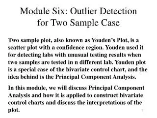
Box Plots of Blood Pressure, Comparing Male and Female The likely outlier, 210 is a Male. The distribution for Male is somewhat skewed-to-right. However, excluding 210, it will be pretty much symmetric. However, there are some potential extremes on either end. The distribution shape for Female is approximately symmetric, and therefore, we can assume Normality for Female.
Hands-on activity Use the Inter-laboratory testing data – the TAPPI data to construct a box plot for GR-Lab35-Mean variable and GR-Lab35-Mean-1 variable. And identify the likely outliers from each variable.
3. Numerical Methods for Detecting Outliers a. Studentized Residuals (as known as CPV’s(Comparative Performance Values), h-statistics in the literature of Inter-laboratory testing studies). b. Deleted Studentized Residuals Consider the TAPPI lab data of sample GR35: Using the notations {y1, y2, y3, …., yn} to represent the n data values, one from each lab. When the same testing procedure is applied and each lab process is under statistical control, the expected testing result should be the same. We will use the notation m for the expected measurement.
A Simple model for describing the one sample testing As we demonstrated in the ‘2 cm drawingactivity’, there is always some uncertainties above and below the true measurement, and that if there is no special causes or systematic bias, the deviations between each lab’s testing result, ei= yi – m, should behave at a random fashion. This suggests that each testing result can be expressed in the following model: yi = m +ei for i = 1,2,3, …., n labs This describe the expected situation in one sample testing. We then use the observed lab testing data to estimate the expected testing result and to investigate the random deviation. By using the sample data, this is what we have: yi = +ei . is the average of all included labs (as known as grand mean). ei is what we call residual. And we also see that average of ei’sis zero.
If the testing result , yi from a lab is likely an outlier, it’s corresponding ei will be far away from the average, 0. Therefore, one can use the residual to detect labs with extreme testing result. • In stead of using the residual, ei, itself (the value depends on the measurement units), we use some standardized form of ei to detect outliers, so that, it will not be measurement dependent. • A classical one is : Standardized ei(as known as CPV as well as h-statistics in inter-laboratory studies): • How to compute standardized ei for each lab? • Compute , the grand mean of all included labs. • Compute ei = yi – • Compute the between-lab variance, s2 and standard deviation, s: • s2 = and • 4. Standardized ei = ei/s
How to use standardized residual (CPV or h-statistic) to detect outliers? • A quick rule : • If standardized residual > 2 or < -2 then it is a possible outlier. Since, based on the normal probability, there is approximately only 2.5% of chance to have a standardized residual > 2 or < -2, respectively. • If standardized residual > 2.6 or < -2.6, then, it is a likely outlier. There is approximately only 0.5% of chance to be > 2.6 or < -2.6, respectively. • NOTE: 2.0 and 2.6 are values from the Z-distribution, N(0,1). f(z) .005 .025 .025 .005 Z -2.576 –1.96 0 1.96 2.576
A more precise rule: • Standardized residual > t(.025, n-1) or < -t(.025, n-1), then, it is a probable outlier. • Standardized residual > t(.005, n-1) or < -t(.005, n-1), then, it is a likely outlier. • NOTE: t(a, n-1) is a value of t-distribution. The standardized residual follows a t-distribution with degrees of freedom n-1 in this case. t-distribution is very similar to Z-distribution. T depends on sample size. When sample size is larger, t is eventually the same as Z. f(t) .005 .025 .025 .005 t -t(.005,n-1) –t(.025,n-1) 0 t(.025,n-1) t(.005,n-1)
A more sensitive measure for detecting outliers: • Deleted Standardized Residual, dj. • The steps for computing this measurement: • Delete the jth case, • then compute and residual ei(j) = yi - for every case, including the jth case. • Compute and s(j) using the (n-1) residuals, excluding jth case. • Compute the deleted standardized residual, dj = ej(j)/s(j) • Repeat the steps 1-3 for cases j = 1,2,3 …., n. • Since the Deleted Standardized residual for the jth observation estimates all quantities with this observation deleted from the data set, the jth observation cannot influence these estimates. Therefore, unusual Y values clearly stand out. It is more sensitive than the classical standardized residual.
How to use the Deleted Standardized Residual to detect outliers? The same quick rule as the standardized residual applies here. However, if we are to be more precise, we need to use the t-distribution. In applying the t-distribution, the degrees of freedom is now (n-2). For most of applications, the rule QUICK RULE is sufficient. Unless the sample size n is very small. A common wisdom is that n < 30 is small. However, for practical reason in outlier detection, it is appropriate to consider n < 20 to be small, and that the t-distribution should be applied. The key issue after detecting the outliers is to find out the possible causes of these outliers.
The h-plot for Inter-laboratory Testing The h-plot plots the CPV values on a two dimensional plot with a center line and upper and lower limits along the X-axis. The X-axis is the Lab ID. The CPV values of replications within each lab, if existed, are grouped together. The Y-axis is the standardized (or deleted studentized residuals). An example is given in the following: 2 0 -2 1 2 3 4 5 6 7 8 9 10 11 12 One may use the more precise t-values for the upper and lower bounds : In this plot, there are 12 labs. Each lab has two replications. The length of each line is the standardized residual (h-value or CPV) or deleted studentized residual.
The h-plot is a graphical view of the standardized residuals or deleted studentized residuals. The same plot is not available in Minitab. However, Minitab does provide all needed numerical measurements. We can create a similar graph using Minitab as well. • The outlier detection using residuals is a very useful tool. In the above case, we consider the simplest model that describe one sample data as y = m + e. This model assumes • Each lab is similar in its operation, • The testing procedure is standardized, • The operators have similar quality, • The testing material is similar. • If any of these assumptions is seriously violated, this model is not adequate. A more complicated model should be considered. The outliers detection should not be applied to response variable directly if we know in advance the violation of these assumptions.
Use Minitab to compute numerical measurements for conducting outlier detection for one sample case • NOTE: This process involves a lot of computations. We do not do this by hand.Here is the steps of using Minitab to compute residuals, standardized residuals, and deleted standardized residual. • The TAPPI study is used for demonstration here. • Create a column of 1’s, say, in C7: • a. Go to Calc, choose ‘Make Patterned Data, select ‘Arbitrary Set of Numbers’, in the Dialog box, enter C7 to store the data, enter ‘1’ in the ‘Arbitrary set of Numbers’, List each value ’87’ times, the sample size, and List the whole sequence ‘1’ times. • Go to Stat, choose Regression, then select ‘Regression’. • In the Dialog box, enter the response variable, say C5, and enter predictors C7, the column with all ‘1’. • Click on ‘Options’, and deselect ‘Fit Intercept’.
Steps- Continued: • Click on ‘Storage’, and select Residuals, Standardized Residuals, Deleted Studentized Residuals, and Fits. Each of these will appear as a column is the worksheet. • Residuals is named: RESI1, • Standardized Residual is named: SRES1, • Deleted Studentized Residual is named:TRES1 • The Fitted Value is named: FITS1. In the one sample case, this is exactly the Grand Mean of all included labs. • The number at the end of each variable will increase by one, such as RESI2, SRES2, for additional storage in the later analysis. • We can change the variable names as we wish.
There are two additional selections in the Regression Procedure: Graphs, Results. • Click on ‘Graphs’, it allows you to conduct graphical detection of these residuals. Choose some graphs as you wish to see. For example, one may choose ‘Standardized’ choose ‘Normal Plot of Residuals’ to conduct a normal probability plot for standardized residuals. • The Graphs will appear in the graph window. • 7. Click on ‘Results’, it allows to choose the amount of computer output as needed. The last one gives the most extensive output. • The results will appear in the Session Window.
Use Minitab to construct the h-plot • Since Minitab does not have the same plot as h-plot shown before, I will demonstrate how to use other procedure to construct a plot that is similar to the h-plot using the TAPPI data. • Go to Stat, choose Control Charts, then select ‘Individuals’. • In the Dialog box, enter ‘SRES1’ into the Variable box (or any variable of interest such as deleted studentized residuals. • Enter 0 for Historical Mean. This will be the center line on the plot. • There are five additional selections and three graph editing selections. Leave Test and Estimate as default. • Click on ‘S-Limit’ selection, and enter 2 for upper sigma limit and –2 for lower sigma limit. You can also change the line color and line type. • Click on ‘Stamp’ selection, enter C1 as the Tick Labels. This will define the ticks on the X-axis using the laboratory names. • Click on ‘Options’ selection, you can change the symbol attributes and connection line attributes.
Case Example: TAPPI Inter-laboratory Study • Let’s start with the SAMPLE GR35. • A quick eye-checking immediately suggest the following cases are clear outliers, and they are removed from the outlier detection analysis immediately: • U3438: Lab mean = 80.55 , U3531: Lab mean = 85.75 • Now, we follow the procedure described above to compute the standardized residuals and deleted studentized residuals using the remaining data and normal plot analysis. • The unusual observations are Unusual Observations • Lab Code GR35-Lab Fit SE Fit Residual St Resid • U2415 1.00 76.0630 77.5273 0.0652 -1.4643 -2.45R • U3154 1.00 79.5500 77.5273 0.0652 2.0227 3.39R • U3185 1.00 79.1000 77.5273 0.0652 1.5727 2.63R • U3216 1.00 79.1620 77.5273 0.0652 1.6347 2.74R • U3249 1.00 76.2630 77.5273 0.0652 -1.2643 -2.12R • U3292 1.00 79.1380 77.5273 0.0652 1.6107 2.70R • U3334 1.00 78.7750 77.5273 0.0652 1.2477 2.09R
The normal probability plot and Normality test for the Standardized Residuals The pattern does not follow a straight line well. The Normality Test suggests the lab testing results clearly do not follow normal.
The quick rule is used to detect the outliers in this case, since the sample size is large. • Both standardized residuals and deleted studentized residuals give the same group of unusual labs. • These labs of which the testing results are found unusual will be notified. Further analysis is then taken to find out if there are any special causes or reasons for these unusual lab results. • NOTE, the result using one sample detection technique is somewhat different from the two-sample plot approach. Since some labs which do not show outliers from this sample may show outliers when testing another sample. This is one reason why we should also conduct two-sample plots.
This is created by Minitab. It is not quite the same as the h-plot. It does the same function as the h-plot and more. The mark ‘1’ is the lab which is over 3, a definite outlier. The labs outside the upper and lower limit of 2 are considered as outlier. One can choose to use different upper and lower bounds.
Hands-on Activity Detect labs which result outliers in testing Sample GR 36 of the TAPPI study.
Use of Basic Quality Control Chart Techniques for monitoring laboratory performances • Quality Control charts were originally developed to monitor the mean shift and and the variation changes along the time domain in manufacturing process. For the inter-laboratory performance of testing a given material, we can apply the same charting method to monitor the performance of laboratories based on two measurements: • laboratory measurement means and • within-lab measurement variations. • The control charts to be discussed are called Example: A study of a chromatographic method was conducted for determining malathion. Ten labs participated in the study; each lab received a subsample of a technical grade malathion (Tech), two wettable powders (25% WP and 50% WP), and an emulsifiable concentrate (58% EC), and a dust. Each participant also received an internally tested standard of malathion (99.1%) along with the analytical method. (Wernimont, 1985).
Row lab Rep WP25 WP50 1 1 1 26.17 50.76 2 1 2 26.22 50.67 3 1 3 25.85 50.81 4 1 4 25.80 50.72 5 2 1 26.44 50.82 6 2 2 26.57 50.90 7 2 3 25.80 51.04 8 2 4 26.06 50.96 9 3 1 26.95 52.53 10 3 2 26.91 52.54 11 3 3 26.98 52.55 12 3 4 26.91 52.47 13 5 1 26.23 50.20 14 5 2 26.00 50.47 15 5 3 26.22 50.39 16 5 4 26.18 50.43 17 6 1 25.45 51.65 18 6 2 25.62 51.67 Row lab Rep WP25 WP50 19 6 3 27.01 51.72 20 6 4 25.72 52.07 21 7 1 26.14 50.53 22 7 2 26.78 50.75 23 7 3 26.04 49.99 24 7 4 25.97 50.92 25 8 1 25.70 50.00 26 8 2 25.90 50.30 27 8 3 25.80 50.50 28 8 4 25.70 50.60 29 9 1 26.13 50.26 30 9 2 26.13 50.36 31 9 3 25.91 50.97 32 9 4 25.86 50.44 33 10 1 26.22 50.23 34 10 2 26.20 50.27 35 10 3 25.84 50.29 36 10 4 25.84 49.97
Construction of Consider the above Malathion testing study. Ten labs particilated in the study. Each Lab tested material WP50 for four replications. Lab 4 was excluded since it did not complete the testing. Range = Largest – Smallest in each Lab.
An X-bar chart is to monitor the laboratory mean. If labs are consistent, then, the average of each lab should be close. If all of them the equal, then, the grand average is the same of lab average. If lab averages are very different (that is some lab systematic biases exist), then there will have deviation between grant mean and lab mean. This provides the basis of the X-bar chart. Upper Limit m Grand Mean Lower Limit Lab order (or Time order) The lab averages are then plotted along the lab order. The multiple ‘3’ is applied commonly in process control. Under the normality assumption, there is 99.7% of chance the lab sample mean should be within the interval. As the chart indicates, we need to estimate the grand mean and SE of lab mean. Since range is usually easier to compute, the estimate of the population variance and, hence the SE of lab mean can also be estimated, using the distribution of Range.
The expected value of Range: E(R) = d2sx , where d2 depends on sample size (in the lab testing case, it is the # of replications conducted by each lab. The values of d2 will be provided in the class. Therefore, the estimate of sx is given by And the SE of sample mean is
Analyzing the malathion data – the WP50 variable • X-bar chart suggests that there exists a very large mean differences among labs. This is an indication of systematic lab bias. When comparing with the standard proportion of 50%, Lab 3 shows much higher lab average than others. Some attention to Lab 3 should be taken. • R-chart indicates, in general, no lab has dramatically high within-lab variation. However, Lab 7 has somewhat higher within-lab variation.
Analyzing the Malathion Data – 25% Variable X-bar chart for the WP25% variable also show that Lab 3 has a significantly high lab average. A closer check is necessary. The R-chart indicates the within-lab variation exceeds the upper limit. A review of Lab 6 for special causes would be recommended.
Some General Comments of applying the control charts for monitoring laboratory means and within-lab variations • This X-bar, R-chart technique is valid under the assumptions: • The response variable follows a normal distribution. • The same or very similar material is tested by every participated lab. • The operation of each lab is independent of others. • In most laboratory studies, • condition (3) is usually satisfied. • Condition (2) may be satisfied if the preparation and distribution of material and the time period of conducting the lab testing is within a reasonable time period. • If there are more than one material tested by participated labs, we can conduct a series of control charts to monitor each material. There are also multivariate control charts that can be applied to monitor more than one material at a time and take into account the laboratory systematic biases into account. • The Youden’s two-sample plots can be applied (to be discussed later) to diagnose the lab performance based on two samples at a time.
Other Control Charts that may be useful for monitoring inter-laboratory testing study
How to use Minitab to conduct control chart analysis? Constructing X-bar and R-charts is straightforward even by hand. However, Minitab can do the charting and much much more for us. There are steps are constructing the X-bar and R-charts: 1. GO to Stat, choose Control Charts, select Xbar-R… 2. In the dialog box, depending on the data arrangement in the worksheet. If response is in one column and lab# in another column, enter response and lab id columns into ‘single column’ and ‘sub-group size’. 3. There are four selections. We have shown these before. Click on ‘Stamp’ selection, and enter the column that consists of the correct ‘Lab ID or Name’ . The correct ID or Lab Name will show on the X-ticks for easier reading.
Hands-on Activity • Analyze the other variables in the Malathion data, and draw your final conclusion about the lab consistency with regards to • Lab averages, • Within-lab variations