Download
1 / 24
240 likes | 504 Vues
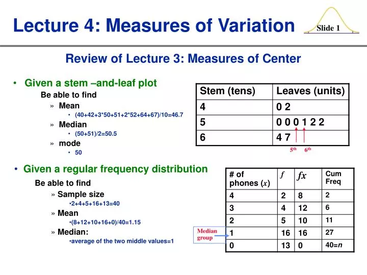
Given a stem –and-leaf plot Be able to find Mean (40+42+3*50+51+2*52+64+67)/10=46.7 Median (50+51)/2=50.5 mode 50. Lecture 4: Measures of Variation. Review of Lecture 3: Measures of Center. 5 th 6 th. Given a regular frequency distribution Be able to find

E N D
Given a stem –and-leaf plot Be able to find Mean (40+42+3*50+51+2*52+64+67)/10=46.7 Median (50+51)/2=50.5 mode 50 Lecture 4: Measures of Variation Review of Lecture 3: Measures of Center 5th6th • Given a regular frequency distribution • Be able to find • Sample size • 2+4+5+16+13=40 • Mean • (8+12+10+16+0)/40=1.15 • Median: • average of the two middle values=1 Median group
2.5 Measures of Variation Measure of Variation (Measure of Dispersion): A measure helps us to know the spread of a data set. Candidates: Range Standard Deviation, Variance Coefficient of Variation Statistics handles variation. Thus this section one of the most important sections in the entire book
The range of a set of data is the difference between the highest value and the lowest value Definition Range=(Highest value) – (Lowest value) Example: Range of {1, 3, 14} is 14-1=13.
Standard Deviation The standard deviation of a set of values is a measure of variation of values about the mean • We introduce two standard deviation: • Sample standard deviation • Population standard deviation
(x - x)2 S= n -1 Formula 2-4 Sample Standard Deviation Formula Data value Sample size
n (x2)- (x)2 s = n (n -1) Formula 2-5 Sample Standard Deviation (Shortcut Formula)
Data: 1, 4, 10. Find the sample mean and sample standard deviation. Example: Publix check-out waiting times in minutes Using the shortcut formula: 1-5= n=3
Standard Deviation - Key Points • The standard deviation is a measure of variation of all values from the mean • The value of the standard deviation s is usually positive and always non-negative. • The value of the standard deviation s can increase dramatically with the inclusion of one or more outliers (data values far away from all others) • The units of the standard deviation s are the same as the units of the original data values
(x - µ) 2 = N Population Standard Deviation This formula is similar to Formula 2-4, but instead the population mean and population size are used
Population variance: Square of the population standard deviation Variance • The variance of a set of values is a measure of variation equal to the square of the standard deviation. • Sample variance s2: Square of the sample standard deviation s
s } 2 Sample variance Notation 2 Population variance Variance - Notation standard deviation squared
Carry one more decimal place than is present in the original set of data. Round-off Rulefor Measures of Variation Round only the final answer, not values in the middle of a calculation.
Sample Population CV = CV = Definition The coefficient of variation (or CV) for a set of sample or population data, expressed as a percent, describes the standard deviation relative to the mean • A measure good at comparing variation between populations • No unit makes comparing apple and pear possible.
Sample: 40 males were randomly selected. The summarized statistics are given below. Example: How to compare the variability in heights and weights of men? Conclusion: Heights (with CV=4.42%) have considerably less variation than weights (with CV=15.26%) Solution: Use CV to compare the variability Heights: Weights:
Use the class midpoints as the x values Formula 2-6 n[(f • x2)]- [(f•x)]2 S= n(n -1) Standard Deviation from a Frequency Distribution
A random sample of 80 households was selected Number of TV owned is collected given below. Example: Number of TV sets Owned by households • Compute: • the sample mean • (b) the sample standard deviation
Range 4 s Estimation of Standard Deviation Range Rule of Thumb For estimating a value of the standard deviation s, Use Where range = (highest value) – (lowest value)
Minimum “usual” value (mean) – 2 X (standard deviation) Maximum “usual” value (mean) + 2 X (standard deviation) Estimation of Standard Deviation Range Rule of Thumb For interpreting a known value of the standard deviation s, find rough estimates of the minimum and maximum “usual” values by using:
Definition Empirical (68-95-99.7) Rule For data sets having a distribution that is approximately bell shaped, the following properties apply: • About 68% of all values fall within 1 standard deviation of the mean • About 95% of all values fall within 2 standard deviations of the mean • About 99.7% of all values fall within 3 standard deviations of the mean
The Empirical Rule FIGURE 2-13
The Empirical Rule FIGURE 2-13
The Empirical Rule FIGURE 2-13
Recap In this section we have looked at: • Range • Standard deviation of a sample and population • Variance of a sample and population • Coefficient of Variation (CV) • Standard deviation using a frequency distribution • Range Rule of Thumb • Empirical Distribution
problems 2.5: 1, 3, 7, 9, 11, 17, 23, 25, 27, 31 Read: section 2.6: Measures of relative standing. Homework Assignment 4