California’s Water WAR: Part II

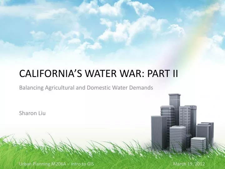
1. California’s Water WAR: Part II Balancing Agricultural and Domestic Water Demands Sharon Liu • Urban Planning M206A – Intro to GISMarch 19, 2012

2. Introduction THE FACTS • California has a significant agriculture industry. • California has a growing population. OUR PROBLEM • Both crops and people need water. • Freshwater is a finite resource. THE FUTURE • Who gets the water when both demands increase? • How will this impact California’s agriculture industry? YEAR 2000 moderate La Niña (dry weather) • SOURCES: Global ENSO SST Index (University of Washington)

3. CROP VALUE: states • SKILLS: graduated symbols, aggregating attribute fields (Crop Value = Field/Misc. Crops + Fruits/Nuts + Commercial Vegetables) • SOURCES: UCLA Mapshare State and Country Boundaries, US Department of Agriculture (2000 Crop Values), 2000 US Census Bureau

4. Crop Value: US vs. Ca in billions ~17% of US total crop value >50% of US crop value for both commercial vegetables and fruits and nuts • SKILLS: EXCEL pie charts • SOURCES: US Department of Agriculture (2000 Crop Values)

5. Population Projections • SKILLS: EXCEL bar chart, inset map, graduated symbols, creating indices (fractional population change) • SOURCES: UCLA Mapshare County, State, and Country Boundaries; California Department of Finance (2000 population & decadal projections)

6. Evaluation METRICS • Agricultural Water Demands • Domestic Water Demands • Irrigation Efficiency (proxied by evapotranspiration) SCALES • Spatial: county • Temporal: monthly, annual, decadal SIMPLIFYING ASSUMPTIONS • Water conservation efforts were not considered. • Climate variability (and climate change) were not considered. • Total available water is fixed. • Other water uses (industrial, thermoelectric, mining, etc) assumed constant. • Freshwater sources and transport (via aqueducts) were not considered.

7. Evapotranspiration Irrigation Efficiency

8. RECALL: What is Evapotranspiration? ET = Evaporation + (Plant) Transpiration Sufficient H20 ↑ crop growth (↑ ET) =↑ crop value($) Where does the H20 come from? • Native (rainfall, groundwater, etc) • Irrigation (imported water)

9. WEATHER Stations • 224 stations total • 94 stations with data for year 2000 Use CIMIS data to calculate ET (Currently, 141 active and 83 inactive) • SKILLS: inset map, original data (CIMIS station locations) • SOURCES: UCLA Mapshare County, State, and Country Boundaries, California Department of Water Resources (2000 Irrigated Crop Acres and Water Use), California Irrigation Management and Information System (station locations and period of record)

10. Monthly Evapotranspiration WINTER SPRING

11. Monthly Evapotranspiration SUMMER FALL 13

12. Statistical Significance • SPATIAL AUTOCORRELATION • z-score = 9.41:>99% likelihood that pattern is NOT random • Moran’s Index = 0.323:values have some correlation • SKILLS: graduated symbols, hot spot analysis, aggregating attribute fields (annual = ∑monthly), model (kriging and clip), analysis (kriging), spatial statistics (spatial autocorrelation [Moran’s Index]) • SOURCES: UCLA Mapshare County, State, and Country Boundaries; California Irrigation Management and Information System (locations and annual ETo)

13. Modeled Evapotranspiration • SKILLS: creating indices (AW Efficiency = ETAW/AW), aggregating attribute fields (Applied Water = ΣAW for all 20 crop types), graduated symbols • SOURCES: UCLA Mapshare County, State, and Country Boundaries, California Department of Water Resources (2000 Irrigated Crop Acres and Water Use)

14. Water Volume and Total Crop Production Value Future Impacts

15. Water Volume: County * Linear projections based on % change in population in each county • SOURCES: UCLA Mapshare County, State, and Country Boundaries; California Department of Water Resources (2000 Irrigated Crop Acres and Water Use)

16. Water Volume: State AGRICULTURAL WATER: Variable • In 2000, 30,497 Mgal/day yielded $15.5 billion. • In 2050, 79,040 Mgal/day could potentially yield $40.1 billion. DOMESTIC WATER: Minimum Required MAX AVAILABLE WATER: Fixed • 36,904 Mgal/day WHICH CROPS GET WATER? • 25,049 Mgal/day is available for agriculture. deficit (53,991) ($??) 25,049 $??

17. Planning Scenarios HOW TO BALANCETHE WATER DEMANDS? Scenario I:Maximize crop production by first watering crops with the highest irrigation efficiency Scenario II:Maximize crop profit by first watering crops with the greatest crop value Scenario III:Maintain crop diversity by applying a proportional reduction in agricultural water Scenario IV:Specialize crops (focus on commercial vegetables and fruits & nuts) by first watering crops with the highest irrigation efficiency

18. Ex. Scenario III: maintain crop diversity Scenario III: Maintain crop diversity by applying a proportional reduction in agricultural water __________________________________ WHICH CROPS GET WATER? • 25,049 Mgal/day is available for agriculture. • Between 2000 and 2050, total crop production value would decrease by $2.4 billion. deficit (53,991) ($27.0) 25,049 $13.1

19. Summary • Freshwater is a finite resource (future demand >> supply). • There are many different approaches on how to allocate the water available for agriculture. • Irrigation Efficiency (using ET) is a statistically significant, yet complicated option. (It also depends on modeled ETAW values.) • Results suggest that there will be a decrease in $$ generated from the agriculture industry.

20. Model Can also be applied to monthly ETo data in California. • SKILLS: model creation (Kriging interpolation of annual precipitation and clipping to California boundary) • SOURCES: UCLA Mapshare County, State, and Country Boundaries; California Department of Water Resources (2000 Irrigated Crop Acres and Water Use)

21. Skills • Model • Measurement/Analysis • Original Data • Inset Map • Graduated symbols • Aggregating attribute fields • Creating indices • Attribute subset selection • Distance • Charts, images • Hotspot Analysis (Spatial Analyst) • Spatial Statistics • Time-based Analysis

22. Questions?