Download
1 / 78
970 likes | 1.57k Vues
6. QUANTUM MECHANICS AND ATOMIC STRUCTURE. CHAPTER. 6.1 Quantum Picture of the Chemical Bond 6.2 Exact Molecular Orbital for the Simplest Molecule: H 2 + 6.3 Molecular Orbital Theory and the Linear Combination of Atomic Orbitals Approximation for H 2 +

E N D
6 QUANTUM MECHANICS AND ATOMIC STRUCTURE CHAPTER 6.1 Quantum Picture of the Chemical Bond 6.2 Exact Molecular Orbital for the Simplest Molecule: H2+ 6.3 Molecular Orbital Theory and the Linear Combination of Atomic Orbitals Approximation for H2+ 6.4 Homonuclear Diatomic Molecules: First-Period Atoms 6.5 Homonuclear Diatomic Molecules: Second-Period Atoms 6.6 Heteronuclear Diatomic Molecules 6.7 Summary Comments for the LCAO Method and Diatomic Molecules General Chemistry I
Potential energy diagram for the decomposition of the methyl methoxy radical
6.1 QUANTUM PICTURE OF THE CHEMICAL BOND • Potential energy of H2 (seesection 3.7) V = Ven + Vee + Vnn • Using effective potential energy function, Veffor V(RAB) - At large RAB, Veff → 0, and the atoms do not interact. - As RAB decreases, Veff must become negative because of attraction. - At very small RAB, Veff must become positive and large as Veff → ∞.
Fig. 6.1 E0 : zero-point energy for the molecule by the uncertainty principle Dissociation energy: Do or De
Changes in electron density on formation of H2 from 2H (Fig. 6.2)
Born-Oppenheimer Approximation: Slow Nuclei, Fast Electrons - Nuclei are much more massive than the electrons, the nuclei in the molecules will move much more slowly than the electrons. → decoupling of the motions of the nuclei and the electrons (A) Consider the nuclei to be fixed at a specific set of positions. Then solve Schrödinger’s equation for the electrons moving around and obtain the energy levels and wave functions. Next, move the nuclei a bit, and repeat the calculation. Continue this procedure in steps. Each electronic energy level (E(el)a) is related to the nuclear coordinates, RAB. (a: the proper set of quantum numbers)
- Visualizing a group of electrons moving rapidly around the sluggish nuclei, to establish a dynamic distribution of electron density (Fig. 6.3). rapid movement of the electrons effective potential energy functions
Mechanism of CovalentBond Formation First phase - When RAB → ∞, independent H atoms e-
- As the two atoms approach one another, Second phase (The ‘particle in a box’ energies decrease as the size of the box increases) e-
- As bond formation continues, Third phase e-
Final phase e-
For the ionic bond, potential energy alone is essential. (section 3.8) repulsion attraction • For the covalent bond, the charge distribution and the kinetic energy of the electrons are also important.
6.2 EXACT MOLECULAR ORBITALS FOR THE SIMPLEST MOLECULE: H2+ • H2+ ion: a single electron bound to two protons • bond length 1.06 Å; bond dissociation energy 2.79 eV = 269 kJ mol-1 - For a fixed value of RAB, the position of the electron: - The potential energy has cylindrical (ellipsoidal) symmetry around the RAB axis.
By the Born-Oppenheimer approximation, - RAB : holding at the equilibrium bond length of 1.06 Å Omitting f due to the same potential energy for all values of f • The solution of the Schrödinger equation: - smooth, single-valued, and finite in all regions of space to define a probability density function of its square Solutions exists when the total energy and angular momentum are quantized.
Electronic Wave Functions for H2+ - isosurface comprising the wave function with 0.1 of its maximum value. - red: + amplitude; blue: - amplitude - molecular orbital: each of exact one-electron wave functions
Molecular orbital nomenclature - Four labels summarize the energy and the shape of each wave function. 1) integer: an index tracking the relative energy of the wave functions of each symmetry type. i.e.) 1sg: the first (the lowest energy) of the sg wave functions 2) Greek letter: how the amplitude of the wave function is distributed around the internuclear axis. - s : the amplitude with cylindrical symmetry around the axis - p : the amplitude with a nodal plane that contains the internuclear axis
3) g or u: how the wave function changes as we invert our point of observation through the center of the molecule (i.e. the wave function at (x, y, z) and (-x, -y, -z): g : symmetric, the same at these points (‘gerade’) u : antisymmetric, the opposite at these points (‘ungerade’) 4) *: how the wave function changes when the point of observation is reflected through a plane perpendicular to the internuclear axis: no * symbol : no changing sign upon reflection (bonding MO) • : changing sign upon reflection (antibonding • MO)
Nature of the Chemical Bond in H2+ antibonding MO bonding MO
Summary of the Quantum Picture ofChemical Bonding for H2+ 1. The Born-Oppenheimer approximation: fixing the nuclei positions 2. Molecular orbital: one-electron wave function, its square describes the distribution of electron density 3. Bonding MO: increased e density between the nuclei decreased effective potential energy 4. Antibonding MO: a node on the internuclear axis high effective potential energy 5. s orbital: cylindrical symmetry; cross-sections perpendicular to the internuclear axis are discs. 6. p orbital: has a nodal plane containing the internuclear axis
6.3 MOLECULAR ORBITAL THEORY AND THE LINEAR COMBINATION OF ATOMIC ORBITALS APPROXIMATION FOR H2+ • LCAO method: selecting sums and differences (linear • combinations) of atomic orbitals to generate the best • approximation to each type of molecular orbital - The general form for H2+
MOs of the s bonding • The distribution of electron probability density
Plots of wave functions and electron probability density for H2+ MOs (Fig. 6.7)
Energy of H2+ in the LCAO Approximation sg1s, RAB = 1.32 Å, D = 1.76 eV 1sg, RAB = 1.06 Å, D0 = 2.79 eV Calculated by Burrau (1927): exact solutions of Schrödinger equation
Correlation diagram: the energy-level diagram within the LCAO-MO model
6.4 HOMONUCLEAR DIATOMIC MOLECULES: FIRST-PERIOD ATOMS For H2 and He2+,
H2: Stabilization of bonding MO • by 2 (–E) for H2 • compared to the • noninteracting system. • He2+: Stabilization of bonding MO by 2 (–E) • compensated by destabilization • of antibonding MO by +E . • Net stabilization energy = • –E
Bond order Bond order = (1/2) x (number of electrons in bonding MOs – number of electrons in antibonding MOs)
6.5 HOMONUCLEAR DIATOMIC MOLECULES: SECOND-PERIOD ATOMS • LCAO-MO approximation • Combination of 2s AOs to form g2s and u2s* MOs • Combination of 2pz AOs to form and MOs
Rules for LCAO-MO Model (Mulliken) 1. Only AOs of the same symmetry along the bond axis can be combined to give MOs. 2. AOs of the same or similar energies will interact more strongly than those of widely different energies.
Fig. 6.14. Formation of (a) bonding and (b) antibonding MOs from 2pz orbitals on atoms A and B.
Determination of energy ordering 1. Average energy of bonding-antibonding pair of MOs similar to that of original AO’s 2. Energy difference between a bonding-antibonding pair becomes large as the overlap of AO’s increases 3. Rule of thumb 1: bonding MOs < antibonding MOs 4. Rule of thumb 2: energy increases with number of nodes 5. Ordering for s-group: s2s < s2s* < s2p < s2p* (see slide 35) 6. Ordering for p-group: p2p <p2p* (see slide 35) 7. For ordering s and p, experimental results must be invoked: p2p < s2p, p2p* < s2p* for all the 2nd-row molecules s2p < p2p for O2 and F2 (see slide 36, etc)
Energy ordering of s and p MO types Energy increases with the no. of nodes in the same symmetry. σ-MOs π-MOs Box wave functions
Fig. 6.16. Energy levels for the homonuclear diatomics Li2 through F2.
Fig. 6.17. Correlation diagrams for second-period diatomic molecules, N2 & F2.
Correlation diagram and corresponding MOs for N2
Correlation diagram and corresponding MOs for F2
Cross-over in the correlation diagrams of Li2~N2 and O2~Ne2 • Reversed ordering of energy for Li2 ~ N2 • ~ Due to large electron-electron spatial repulsions between • electrons in and MO’s. • Normal ordering of energy for O2, F2, Ne2 • ~As Z increases, the repulsion decreases since electrons • in MO’s are drawn more strongly toward • the nucleus. 40
Fig. 6.18. (a) Paramagnetic liquid oxygen, O2, and (b) diamagnetic liquid nitrogen, N2, pours straight between the poles of a magnet.
Fig. 6.19. Trends in several properties with the number of valence electrons in the second-row diatomic molecules.
6.6 HETERONUCLEAR DIATOMIC MOLECULES For the 2s orbitals, s2s = CA2sA + CB2sB s2s* = CA’2sA – CB’2sB In the homonuclear case, CA = CB; CA’ = CB’ If B is more electronegative than A, CB > CA for bonding s MO, CA’ > CB’ for the higher energy s* MO, closely resembling a 2sA AO
B O Fig. 6.20. Correlation diagram for heteronuclear diatomic molecule, BO. (O is more electronegative) LCAO/MO electron configuration: (s2s)2(s*2s)2(p2px)2(p2py)2(s2pz)1
Fig. 6.22. Correlation diagram for HF. The 2s, 2px, and 2py atomic orbitals of F do not mix with the 1s atomic orbital of H, and therefore remain nonbonding. LCAO/MO electron configuration:
s +1sH +2pFz Fig. 6.21. Overlap of atomic orbitals in HF. (d) pnb +1sH +2pFx,y (c) +1sH –2pFz s* (b) snb ((a) +1sH +2sF (a)
6.7 SUMMARY COMMENTS FOR THE LCAO-MO METHOD AND DIATOMIC MOLECULES The qualitative LCAO-MO method easily identifies the sequence of energy levels for a molecule, such as trends in bond length and bond energy, but does not give their specific values. The qualitative energy leveldiagram is very useful for interpreting experiments that involve adsorption and emission of energy such as spectroscopy, ionization by electron removal, and electron attachment.
6.8 VALENCE BOND THEORY AND THE ELECTRON PAIR BOND • Explains the Lewis electron pair model • VB wave function for the bond is a product of two • one-electron AOs • Easily describes structure and geometry of bonds • in polyatomic molecules
Single Bonds - At very large values of RAB, independent atoms - As the atoms begin to interact strongly, indistinguishable
VB wave function for the single bond in a H2 molecule Fig. 6.24. (a) The electron density g for gel and u for uel in the simple VB model for H2. (b) Three-dimensional isosurface of the electron density for the gel wave function in the H2 bond.