Download
1 / 72
720 likes | 745 Vues
Unconfined Aquifer Water Table: Subdued replica of the topography Hal Levin demonstration. after Fetter http://www.uwsp.edu/water/portage/undrstnd/aquifer.htm. Aquifer Types.

E N D
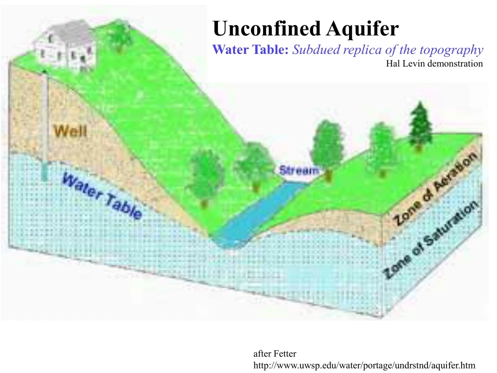
Unconfined Aquifer Water Table: Subdued replica of the topography Hal Levin demonstration after Fetter http://www.uwsp.edu/water/portage/undrstnd/aquifer.htm
Aquifer Types Unconfined Aquifer: aquifer in which the water table forms upper boundary. “Water table aquifer” Head h = z P = 1 atm e.g., Missouri, Mississippi & Meramec River valleys Hi yields, good quality Ogalalla Aquifer (High Plains aquifer): CO KS NE NM OK SD QT Sands & gravels, alluvial apron off Rocky Mts. Perched Aquifer: unconfined aquifer above main water table; Generally above a lens of low-k material. Note- there also is an "inverted" water table along bottom! Confined Aquifer: aquifer between two aquitards. = Artesian aquifer if the water level in a well rises above aquifer = Flowing Artesian aquifer if the well level rises above the ground surface. e.g., Dakota Sandstone: east dipping K sst, from Black Hills- artesian) Hydrostratigraphic Unit: e.g. MO, IL C-Ord sequence of dolostone & sandstone capped by Maquoketa shale
Dissolved Solids mg/l Cambrian-Ordovician aquifer http://capp.water.usgs.gov/gwa/ch_d/gif/D112.GIF
USGS http://capp.water.usgs.gov/gwa/ch_d/gif/D112.GIF
Typical Yields of Wells in the principal aquifers of the three principal groundwater provinces USGS 1967 Alluvial Valleys & SE Lowland Osage & Till Plains Springfield Plateau Ozark Aquifer St. Francois Aquifer <--Maquoketa Shale <--Davis/Derby-Doe Run 0 500 gpm
Sy = Specific yieldUnits: dimensionless = storativity for an unconfined aquifer "unconfined storativity" = Vol of H2O drained from storage/total volume rock (D&S, p. 116) = Vol of H2O released (grav. drained) from storage/unit area aquifer/unit head drop Sy = Vwd/VT Typically, Sy = 0.01 to 0.30 F&C, p. 61 Specific retention: Sr = f = Sy + Sr + unconnected porosity Ss = specific storageUnits: 1/length = Volume H2O released from storage /unit vol. aquifer /unit head drop (F&C p. 58) Ss = r g (B + f b)whereB= aquifer compressibility ~ 10-5 /m for sandy gravelb = water compressibility f = porosity
Storativity S Units: dimensionless S = Volume water/unit area/unit head drop = "Storage Coefficient" S = m Ss confined aquifer S = Sy + m Ss unconfined; note Sy >> mSs For confined aquifers, typically S = 0.005 to 0.00005 Transmissivity T = K*m m = aquifer thickness Units m2/sec = Rate of flow of water thru unit -wide vertical strip of aquifer under a unit hyd. Gradient T ≥ 0.015 m2/s in a good aquifer
HYDRAULIC DIFFUSIVITY (D): Freeze & Cherry p. 61 D = T/S Transmissivity T /Storativity S = K/Ss Hydraulic Conductivity K/ Specific Storage Ss
FUNDAMENTAL CONCEPTS AND PARTIAL DERIVATIVES Scalars: Indicate scale (e.g., mass, Temp, size, ...) Have a magnitude Vectors: Directed line segment, Have both direction and magnitude; e.g., velocity, force...) v = f i + g j + h k where i, j, k are unit vectors Two types of vector products: Dot Product (scalar product): a. b = b. a= |a| |b| cosg commutative Cross Product (vector product): a x b = - b x a = |a| |b| sing anticommutative i. i = 1 j. j = 1 k. k = 1 i. j = i. k = j. k = 0 Scalar Field: Assign some magnitude to each point in space; e.g. Temp Vector Field: Assign some vector to each point in space; e.g. Velocity
FUNCTIONS OF TWO OR MORE VARIABLES Thomas, p. 495 There are many instances in science and engineering where a quantity is determined by many parameters. Scalar function w = f(x,y) e.g., Let w be the temperature, defined at every point in space Can make a contour map of a scalar function in the xy plane. Can take the derivative of the function in any desired direction with vector calculus (= directional derivative). Can take the partial derivatives, which tell how the function varies wrt changes in only one of its controlling variables. In x direction, define: In y direction, define:
FUNCTIONS OF TWO OR MORE VARIABLES Thomas, p. 495 There are many instances in science and engineering where a quantity is determined by many parameters. Scalar function w = f(x,y) e.g., Let w be the temperature, defined at every point in space Define the Gradient: “del operator” The gradient of a scalar function w is a vector whose direction gives the surface normal and the direction of maximum change. The magnitude of the gradient is the maximum value of this directional derivative. The direction and magnitude of the gradient are independent of the particular choice of the coordinate system.
If the function is a vector (v) rather than a scalar, there are two different types of differential operations, somewhat analogous to the two ways of multiplying two vectors together {i.e. the cross (vector) and dot (scalar) products}: Type 1: the curl of v is a vector: Type 2: the divergence of v is a scalar: So: Great utility for fluxes & material balance
dz dy dx Significance of Divergence Measure of stuff in - stuff out Overall Difference Rate of Gain in box
Laplacian: Gauss Divergence Theorem: where un is the surface normal
Continuity Equation (Mass conservation): A = source or sink term; f = flow porosity Steady Flow No sources or sinks Steady, Incompressible Flow r = constant Because the Mass Flux qm :
Continuity Equation (Mass conservation): A = source or sink term; f = flow porosity where Ss = specific storage So, “Diffusion Equation”
“Diffusion Equation” Cartesian Coordinates Cylindrical Coordinates Cylindrical Coordinates, Radial Symmetry ∂h/∂f = 0 Cylindrical Coordinates, Purely Radial Flow ∂h/∂f = 0 ∂h/∂z = 0
Derivative of Integrals: Thomas p. 539 CRC Handbook
“del operator” Gradient: Divergence: Diffusion Equation:
Darcy's Law: Hubbert (1940; J. Geol. 48, p. 785-944) = (k/n)[force/unit mass] • where: • qv Darcy Velocity, Specific Discharge • or Fluid volumetric flux vector (cm/sec) • k= permeability (cm2) • K = kg/n hydraulic conductivity (cm/sec) • Kinematic viscosity, cm2/sec
If fdx +gdy+hdz is an “exact differential” (= du), then it is easy to integrate, and the line integral is independent of the path: Exact differential: If true: Condition for exactness: => Curl u = 0
Conservative Forces Suppose that force F = fi +gj + hk acts on a line segment dl = idx+jdy+kdz : If fdx + gdy + hdz is exact, then the work integral is independent of the path, and F represents a conservative force field that is given by the gradient of a scalar function u (= potential function). In general: 1. Conservative forces are the gradients of some potential function. 2. The curl of a gradient field is zero i.e., Curl (grad u) = 0
Flow Nets: Set of intersecting Equipotential lines and Flowlines Flowlines= Streamlines = Instantaneous flow directions Pathlines= Actual particle path Pathlines ≠ Flowlines for transient flow Flowlines | to Equipotential surface if K is isotropic Can be conceptualized in 3D
No Flow No Flow No Flow Fetter
Flow Net Rules: No Flow boundaries are perpendicular to equipotential lines Flowlines are tangent to such boundaries (// flow) Constant head boundaries are parallel to and equal to the equipotential surface Flow is perpendicular to constant head boundary
Flow beneath Dam Vertical x-section Flow toward Pumping Well, next to river = line source = constant head boundary Plan view River Channel Domenico & Schwartz (1990)
Topographic Highs tend to be Recharge Zones h decreases with depth Water tends to move downward => recharge zone Topographic Lows tend to be Discharge Zones h increases with depth Water will tend to move upward => discharge zone It is possible to have flowing well in such areas, if case the well to depth where h > h@ sfc. Hinge Line: Separates recharge (downward flow) & discharge areas (upward flow). Can separate zones of soil moisture deficiency & surplus (e.g., waterlogging). Topographic Divides constitute Drainage Basin Divides for Surface water e.g., continental divide Topographic Divides may or may not be GW Divides
MK Hubbert (1940) http://www.wda-consultants.com/java_frame.htm?page17
Equipotential Lines Lines of constant head. Contours on potentiometric surface or on water tablemap => Equipotential Surface in 3D Potentiometric Surface: ("Piezometric sfc") Map of the hydraulic head; Contours are equipotential lines Imaginary surface representing the level to which water would rise in a nonpumping well cased to an aquifer, representing vertical projection of equipotential surface to land sfc. Vertical planes assumed; no vertical flow: 2D representation of a 3D phenomenon Concept rigorously valid only for horizontal flow w/i horizontal aquifer Measure w/ Piezometers= small dia non-pumping well with short screen- can measure hydraulic head at a point (Fetter, p. 134)
Effect of Topography on Regional Groundwater Flow after Freeze and Witherspoon 1967 http://wlapwww.gov.bc.ca/wat/gws/gwbc/!!gwbc.html
Saltwater Intrusion Saltwater-Freshwater Interface: Sharp gradient in water quality Seawater Salinity = 35‰ = 35,000 ppm = 35 g/l NaCl type water rsw = 1.025 Freshwater < 500 ppm (MCL), mostly Chemically variable; commonly Na Ca HCO3 water rfw = 1.000 Nonlinear Mixing Effect: Dissolution of cc @ mixing zone of fw & sw Possible example: Lower Floridan Aquifer: mostly 1500’ thick Very Hi T ~ 107 ft2/day in “Boulder Zone” near base,f~30% paleokarst? Cave spongework
PROBLEMS OF GROUNDWATER USE • Saltwater Intrusion • Mostly a problem in coastal areas: GA NY FL Los Angeles • Abandonment of freshwater wells; e.g., Union Beach, NJ • Los Angeles & Orange Ventura Co; Salinas & Pajaro Valleys; Fremont • Water level have dropped as much as 200' since 1950. • Correct with artificial recharge • Upconing of underlying brines in Central Valley
Union Beach, NJ Water Level & Chlorinity Craig et al 1996
Fresh Water-Salt Water Interface? Air Fresh Water r=1.00 hf Sea level ? ? ? Salt Water r=1.025
Ghyben-Herzberg hf Sea level Fresh Water interface z z Salt Water P
Ghyben-Herzberg Analysis Hydrostatic Condition P - rg = 0 No horizontal P gradients Note: z = depth rfw = 1.00 rsw= 1.025
Ghyben-Herzberg hf Sea level Fresh Water interface z z Salt Water P
Physical Effects Tend to have a rather sharp interface, only diffuse in detail e.g., Halocline in coastal caves Get fresh water lens on saline water Islands: FW to 1000’s ft below sea level; e.g., Hawaii Re-entrants in the interface near coastal springs, FLA Interesting implications: If is 10’ ASL, then interface is 400’ BSL If decreases 5’ ASL, then interface rises 200’ BSL 3) Slope of interface ~ 40 x slope of water table
Hubbert’s (1940)Analysis Hydrodynamiccondition with immiscible fluid interface 1) If hydrostatic conditions existed: All FW would have drained out Water table @ sea level, everywhere w/ SW below 2) G-H analysis underestimates the depth to the interface Assume interface between two immiscible fluids Each fluid has its own potential h everywhere, even where that fluid is not present! FW potentials are horizontal in static SW and air zones, where heads for latter phases are constant
… . .. Ford & Williams 1989
Fresh Water Equipotentials … . .. Fresh Water Equipotentials after Ford & Williams 1989