Download
1 / 14
140 likes | 281 Vues
Numerically constrained one-dimensional interaction of a propagating planar shock wave. A. Chatterjee. Department of Aerospace Engineering, Indian Institute of Technology, Bombay Mumbai 400076, INDIA. Shock Wave. u(x, t). u c (x, t). x 2. x 1. x sw.

E N D
Numerically constrained one-dimensional interaction of a propagating planar shock wave A. Chatterjee Department of Aerospace Engineering, Indian Institute of Technology, Bombay Mumbai 400076, INDIA
Shock Wave u(x, t) uc(x, t) x2 x1 xsw 1D problem – numerically constrained interaction of a propagating planar shock wave • Rightward planar propagating shock wave • uc(x, t) : arbitrary imposed flowfield downstream of shock wave • constrains development of flowfield (u(x,t)) behind • propagating shock wave • xsw : currentposition of shock wave
uc (x , x > xsw( t t + t ) t + t ) u( x , t+ t) = t + t ) H[u(x, t)] x < xsw ( x1 < x < x2 uc (x,t) =constraining flowfield downstream of movingshock wave xsw( t + t ) x1 < xsw( t + t ) < x2 = Position of shock wave in [x1 , x2] at obtained from a pressure based sensor = Explicit solution in [x1 , x2] at H[u(x, t)] (3rdorder ENO and 2nd order TVD Runge-Kutta) (t + t ) (t + t ) (t + t ) Algorithm: Proposed algorithm : Unsteady 1D Euler equations in [x1 , x2] :
Vl x < - 4 V(x,0) = x Vr x - 4 [-5 : 5] Vr=(rr,ur,pr)=(1+ 0.2sin(5x), 0, 1) Validation: Test Case: Constrained Interaction of Planar (rightward) Propagating Shock wave • Unsteady interaction of Mach 3 shock wave with Sine entropy wave • (Shu & Osher) Initial Conditions: Vl=(rl,ul,pl)=(3.8571143, 2.629369, 10.333333)
t + t t + t t + t ( rc(x, ), uc(x, ), pc(x , ) ) = ( 1+0.2sin(5x), 0, 1 ) ( t + t ) x > xsw u( x , t+ t) = H[u(x, t)] = H[u(x, t)] u( t + t ) ( t + t ) x xsw Solution Methodologies: Without Constrain (regular solution) in [-5 : 5] With Constrain
Numerical Validation: Shock/entropy wave interaction( time=1.8)
Numerical Validation: Shock/entropy wave interaction( time=1.8)
r Umax U(r) = 0 < r < r1 r1 B U(r) = Ar + r1 rr2 r Application: 2D Shock-vortex interaction problem An initially planar shock wave interacts with a 2D compressible vortex superposed on ambient resulting in creation of acoustic waves and secondary shock structures. ( Compressible vortex model ) Experimental Condition: (Dosanjh & Weeks, 1965) Ms = 1.29 Umax= 177 m/s (Mv=0.52) r1 = 0.277 cm r2= 1.75 cm Strong interaction with secondary shock formation
uc (x) . x1 x2 xsw Application:a possible “constrained numerical experiment”: • Solving numerically a reduced model of complex unsteady shock wave • phenomenon with appropriate constrains • Demonstrate role of purely translational motion of an initially planar shock • wave in secondary shock structure formation when interacting with 2D • compressible vortex • Planar shock wave interact with 1D flow field (uc) • uc represents initial flowfield along vortex model normal to shock wave
Application ….. • uc controls development of the flowfield behind shock wave (example of an • arbitrary constraining flowfield) • Ignores shock wave (and vortex) deformation Computational Domain: [ 0, 20] Initial position of shock = 8. 25 cm Properties behind the shock : R-H condition No. of cells : 900 equally spaced uc constraining flowfield ahead of shock centered at 10.0 cm
uc downstream of normal shock Case 1 & 2 : y 0.45 Case 3 & 4 : y 1.25 Vortex center y=0.0 Velocity distribution along horizontal lines (cases 1 to 4)
Results: Case 1 & 2 : 1.25 (farther from vortex center) T1 = Start of the simulation T6 = Shock wave almost out of domain Pressure Profiles (Case 1) generation of acoustic waves Pressure Profiles (Case 2)
Results: Case 3 & 4 : 0.45 (near vortex center) Pressure Profiles (Case 3) generation of upstream moving shocklet Pressure Profiles (Case 4)
Conclusions: • An algorithm proposed for constrained one dimensional interaction of a planar propagating shock wave. • Validated for 1D shock-entropy wave interaction. • Constraining flowfield can be “arbitrary”. • Allows setting up a “constrained numerical experiment” otherwise not possible.