Download
1 / 30
300 likes | 376 Vues
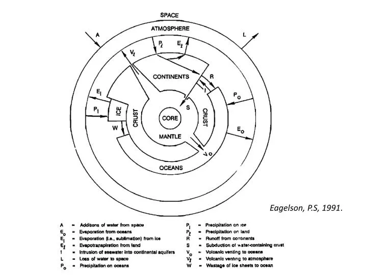
Eagelson , P.S, 1991 . Evap. ANNUAL GLOBAL FLUX 577. All Blue figures in thousands of km 3. ATMOSPHERE. Precip . 12.9. 0.001%. 16%. 84%. 23%. 77%. OCEANS. CONTINENTS. 1,338,000. 47,660. Global Runoff 7%. 97%. 2.999%. +7%. -7%. ATMOSPHERE. 484.7. 12.9. 92.3. 444.3.

E N D
Evap. ANNUAL GLOBAL FLUX 577 All Blue figures in thousands of km3. ATMOSPHERE Precip. 12.9 0.001% 16% 84% 23% 77% OCEANS CONTINENTS 1,338,000 47,660 Global Runoff 7% 97% 2.999% +7% -7%
ATMOSPHERE 484.7 12.9 92.3 444.3 132.7 OCEANS CONTINENTS 1,338,000 47,660 40.4
WATER BALANCE APPROACH Input = Output +/- Change in Storage List List List
WHAT ARE RESIDENCE TIMES? Input = Output ………. No change in Storage Volume of Store = 10 balls Output = 1 ball per time period Input = 1 ball per time period ? ? Average number of samplings required
CHANGE VOLUME OF STORE Volume of Store = 20 balls Output = 1 ball per time period Input = 1 ball per time period ? ?
CHANGE RATES OF INPUT AND OUTPUT Volume of Store = 10 balls Output = 2 balls per time period Input = 2 balls per time period ? ? ? ?
2760 yr = 1,338,000,000 (km3)/ 484,680 (km3 yr-1) Basic time step over which we are completing the accounting.
Volume = 47,659,600 km3 Input rate = Precipitation (23%) Output rate = Evaporation (16%) + Runoff (7%) Average rate = (23 + (16+7))/2 = 23% of 577,000 132,710 km3 per year Avg. Residence = 47,659,600 / 132,710 = 359 years
Volume = 12,900 km3 Input rate = Evap (oceans) (84%) + Evap (continents) (16%) Output rate = Prec. (oceans) (77%) + Prec. (continent) (23%) Average rate = ((84+16) + (77 +23))/2 = 100% of 577,000 577,000 km3 per year Avg. Residence = 12,900 / 577,000 = 0.02 yrs (7.3 days)
GLOBAL SIGNIFICANCE OF RESIDENCE TIMES 2. Rising air cools and vapor condenses, releasing energy to atmosphere and forming clouds. Under the correct conditions, the water drops formed will descend under the influence of gravity (kinetic energy) onto the landscape. 1. Evaporation driven by energy from the Sun, raises water vapor into the atmosphere, renewing the potential energy of the water, and removing most of the dissolved materials inn the water 3. Water moving over and through the landscape uses both its kinetic energy and propensity to dissolves chemicals, to shape the landscape. Rivers, glaciers, caves, groundwater etc. 4. This kinetic and chemical energy given to the water by the Sun, through the process of evaporation is lost once it reaches sea level or some local “datum”, like a lake.
WHICH STORES CONSIDERED WHEN? Unless huge lakes or glaciers present Time and Space scales of studies usually related. Small area , short time step, large area, along time step The shorter the smaller the time step (hour, day, month, year) over which you are accounting, the more stores need to be considered
IMPACT OF LONG-LASTING STORE ST. MARY’S RIVER, SW. PIER, MICHIGAN
Stow, Lamon, Kratz and Sellinger, 2008. Eos, 89, 41, p. 389-390
WATER BALANCE EQUATION • ON A CONTINENTAL SCALE • Input = Output +/- Change in Storage • Precipitation = { Evaporation + Runoff } +/ Change in Storage • Assume ΔS 0 in Long Run Source: Shiklomanov (1990)
MEASURES OF GLOBAL VARIABILITY IN FLOW . Coefficient of Variation = standard deviation/mean Big value represents relatively high variability from year to year (inter-annual variability) • Source: McMahon, T. A., B. L. Finlayson, A. T. Haines, and R. Srikanthan, • 1992: Global Runoff—Continental Comparisons of Annual • Flows and Peak Discharges. Catena Verlag Paperback, 166 pp
MEASURES OF GLOBAL VARIABILITY IN FLOW . Ratio of the discharge of the biggest flow in a year to the average flow in the entire year. Big values mean that the biggest flow with in a year (intra-annual) tend to be extremely large in comparison to the other flow • Source: McMahon, T. A., B. L. Finlayson, A. T. Haines, and R. Srikanthan, • 1992: Global Runoff—Continental Comparisons of Annual • Flows and Peak Discharges. Catena Verlag Paperback, 166 pp
MEASURES OF GLOBAL VARIABILITY IN FLOW . • Source: McMahon, T. A., B. L. Finlayson, A. T. Haines, and R. Srikanthan, • 1992: Global Runoff—Continental Comparisons of Annual • Flows and Peak Discharges. Catena Verlag Paperback, 166 pp
Higher Mean; Higher Variability P R = P - E Land Use Land Cover Lower Mean; Lower Variability Lower Mean; High Variability E R
JONGLEI = DRAINING THE EVERGLADES? Pielke 2001