Download
1 / 54
550 likes | 745 Vues
STAT E-150 Statistical Methods. Review of Statistical Models and Linear Regression Concepts. Statistical Models are used to make predictions, understand relationships, and assess differences. A statistical model can be written as Data = model + error, or Y = f(x) + ε

E N D
STAT E-150Statistical Methods Review of Statistical Modelsand Linear Regression Concepts
Statistical Models areused to make predictions, understand relationships, and assess differences. A statistical model can be written as Data = model + error, or Y = f(x) + ε where Y is the response variable xis the explanatory variable εis the error The error term, ε, represents the part of the response variable that is not explained by its relationship to the predictor variable. We often consider the probability distribution of this error term as part of our assessment of the model.
The Four-Step Process for statistical modeling: • Choose a form for the model Identify the variables and their types • Examine graphs to help identify the appropriate model • 2. Fit the model to the data • Use the sample data to estimate the values of the model parameters • 3. Assess how well the model fits the data • Compare models • Examine the residuals • 4. Use the model to make predictions, explain relationships, assess differences • The appropriate model depends on the type of variables and the role each variable plays in the analysis.
Example: Medical researchers have noted that adolescent females are more likely to deliver low-birthweight babies than are adult females. Because LBW babies tend to have higher mortality rates, studies have been conducted to examine the relationship between birthweight and the mother’s age. One such study is discussed in the article “Body Size and Intelligence in 6-Year-Olds: Are Offspring of Teenage Mothers at Risk?” (Maternal and Child Health Journal [2009], pp. 847-856.)
The following data is consistent with summary values given in the article, and with data published by the National Center for Health Statistics: What are the observational units? Teenage mothers and their babies Which is the response variable? The baby’s weight (in grams) Which is the explanatory variable? The mother’s age (in years)
The following data is consistent with summary values given in the article, and with data published by the National Center for Health Statistics: What are the observational units? Teenage mothers and their babies Which is the response variable? The baby’s weight (in grams) Which is the explanatory variable? The mother’s age (in years)
Simple Linear Regression is used to investigate whether there is a linear relationship between two quantitative variables. If a linear relationship exists, we can create a model for the relationship, and use this model to answer these questions: • What is the relationship between the variables? • What does the slope of this linear model tell us? • When is it appropriate to use this linear model to make predictions?
A First-Order Linear Model is of the form • y = β0 + β1x + ε • where • y = the response variable • x = the independent, or predictor, or explanatory variable • ε = the random error • β0 = where the regression line crosses the y-axis; • the y-intercept of the regression line is the point (0, β0 ) • β1 = the slope of the regression line
Steps in regression Hypothesize the form of the model for E(y), the mean or expected value of y Collect the sample data Use the sample data to estimate the unknown parameters in the model. Specify the probability distribution of ε and estimate any unknown parameters in the distribution. Check the validity of the assumptions made about the probability distribution. Statistically check the usefulness of the model If the model is useful, use the model for appropriate prediction and estimation
Notation: Recall that Data = model + error, or Y = f(x) + ε μy (or μy|x) is the mean value of y for a particular value of x εis the deviation from that mean value at a value of x In a simple linear regression model: μy= f(x) = β1x + β0 (the mean value of y at a given value of x) and y = f(x) + ε = β1x + β0 + ε (the actual value of y for a given x)
In our example, μbirthweight= β1age + β0 The actual birthweights are represented by Birthweight = β1age + β0 + ε
The first step in determining whether there is a linear relationship between the variables is to create a scatterplot of the data, with the explanatory variable on the x-axis and the response variable on the y-axis.
Does there appear to be a linear relationship? What does the scatterplot tell you about the strength and direction of the linear relationship? Write your answer in the context of the scenario.
Does there appear to be a linear relationship?The scatter diagram shows a positive linear relationship What does the scatterplot tell you about the strength and direction of the linear relationship? Write your answer in the context of the scenario.
What does the scatterplot tell you about the strength and direction of the linear relationship? Write your answer in the context of the scenario. The scatter diagram shows that there is a fairly strong positive linear relationship between the two variables: as the mother’s age increases, the child’s birthweight also increased. That is, higher birthweights are associated with older mothers.
Fitting a Simple Linear Model If the data appears to show a linear relationship, the method of least squares finds the line that best fits the data. That is, it will provide the best estimates for β0 and β1. We can find the vertical distance between the observed value of y and the predicted value of y for each value of x. This difference is called the residual:
The points should be scattered about a straight line, with deviations from the line determined by ε. This vertical distance between the observed value of y and the predicted value of y is called the residual. Residual = observed value - predicted value
We want the size of the residuals to be as small as possible; since some residuals are positive and some are negative, we square the residuals and minimize the squares. SSE, the sum of squared errors, is a measure of how well the line predicts the actual values. The Least Squares line is the line where and SSE is minimized. The equation of the least squares line is y = β1x + β0
Some notation: Consider the ith value in the dataset: yi = β0 + β1xi + εi β0 and β1 are the true population values for the population; these are parameters are estimates of the coefficients based on the sample data; these are statistics.
In our example, the equation of the least squares line is weight = 245.15 age – 1163.45 What does the value 245.15represent, in context? What does the value -1163.45 represent, in context?
In our example, the equation of the least squares line is weight = 245.15 age – 1163.45 What does the value 245.15represent, in context? The childs’s birthweight is expected to increase by 125.15g for each additional year in the age of the mother. What does the value -1163.45 represent, in context? If the mother’s age is 0 years, the child’s birthweight is expected to be -1163.45 g.
In our example, the equation of the least squares line is weight = 245.15 age – 1163.45 What does the value 245.15represent, in context? The childs’s birthweight is expected to increase by 125.15g for each additional year in the age of the mother. What does the value -1163.45 represent, in context? If the mother’s age is 0 years, the child’s birthweight is expected to be -1163.45 g.
In our example, the equation of the least squares line is weight = 245.15 age – 1163.45 What birthweight would you expect for the baby of a mother who is 16 years old? weight = 245.15 age – 1163.45 = 245.15(16) – 1163.45 = 3922.4 – 1163.45 = 2758.95 What was the birthweight for the baby of a mother who was 16 years old? 2897 g What is the residual? 2897 – 2758.95g
In our example, the equation of the least squares line is weight = 245.15 age – 1163.45 What birthweight would you expect for the baby of a mother who is 16 years old? weight = 245.15 age – 1163.45 = 245.15(16) – 1163.45 = 3922.4 – 1163.45 = 2758.95 What was the birthweight for the baby of a mother who was 16 years old? 2897 g What is the residual? 2897 – 2758.95g
In our example, the equation of the least squares line is weight = 245.15 age – 1163.45 What birthweight would you expect for the baby of a mother who is 16 years old? weight = 245.15 age – 1163.45 = 245.15(16) – 1163.45 = 3922.4 – 1163.45 = 2758.95 What was the birthweight for the baby of a mother who was 16 years old? 2897 g What is the residual? 2897 – 2758.95g
In our example, the equation of the least squares line is weight = 245.15 age – 1163.45 What birthweight would you expect for the baby of a mother who is 16 years old? weight = 245.15 age – 1163.45 = 245.15(16) – 1163.45 = 3922.4 – 1163.45 = 2758.95 What was the birthweight for the baby of a mother who was 16 years old? 2897 g What is the residual? 2897 – 2758.95 = 138.05g
In our example, the equation of the least squares line is weight = 245.15 age – 1163.45 What birthweight would you expect for the baby of a mother who is 11 years old?
Conditions for a Simple Linear Model • Linearity - the scatterplot shows a general linear pattern • Zero Mean - the distribution of the errors is centered at zero • Constant Variance - the variability of the errors is the same for all values of the predictor variable • Independence - the errors are independent of each other
Conditions for Inference also include: • Random - the data was obtained through a random process • Normality - the distribution of the errors is approximately Normal
More about Residuals: A residual plot is a scatterplot of the regression residuals against the explanatory variable. Residual plots help us assess the fit of a regression line. Here are examples of residual plots: This residual plot shows no systematic pattern; it shows a uniform scatter of the points about the fitted line, and indicates that the regression line fits the datawell.
A curved pattern shows that the data is not linear, so a straight line is not a good fit for the data. This residual plot shows that there is more spread for larger values of the explanatory variable, indicating that predictions will be less accurate when x is large. You should also note any values with large residuals. These points are outliers in the vertical (y) direction because they lie far from the line that describes the overall pattern.
The Simple Linear Regression Model For a quantitative response variable Y and a single quantitative explanatory variable X the simple linear regression model is Y = β0 + β1 X + β0 + ε where ε follows a normal distribution, that is ε ~ N(0, σε) and the errors are independent from one another.
Assessing Conditions To check the Linearity Condition, consider a scatterplot of the data to see if the points suggest a linear relationship.
Assessing Conditions Check the Constant Variance Condition with a plot of the residuals. Graphs of the residuals can also help to determine whether the conditions are met.
This tells us that the slope of the regression line is -3.23 and the y-intercept is the point (0, 1676.4). And so the equation of the regression line is Mortality = -3.23 calcium + 1676.4
Mortality = -3.23 calcium + 1676.4 In other words, if the calcium level increases by one ppm, the mortality rate is expected to decrease by 3.23 deaths per 100,000, on average. The y-intercept tells us that if the calcium level is 0 ppm, the mortality rate would be 1676 deaths per 100,000. However, in this case, this would be an extrapolation.
To add the graph of the regression line to the scatterplot: > plot(x,y) > abline(name of model) For our data, these commands produced this graph: > plot(calcium, mortality) > abline(model)
Making Predictions; Interpolation and Extrapolation The linear model makes it possible to make reasonable predictions about any mean response within the range of the explanatory variable. Statements about the mean at values of the explanatory variable not in the data set but within the range of the observed values are called interpolations. Making predictions for values outside of the range of the data is called extrapolation and is not necessarily valid.
To make a prediction: First create a data structure called a dataframe that contains the value(s) of the explanatory variable that you want to use in your prediction; you may use any appropriate name: >newdata=data.frame(predictor=value) Then attach this new value to make it available to R: >attach(newdata)
Now you can make your prediction. You may choose to include these arguments: - a confidence interval or a prediction interval (default = none) - level of confidence (default is .95) > predict (model, newdata, interval=”confidence”, level=.95)
Example: Predict the mortality rate in a town where the hardness level of the water is 105 ppm of calcium. > newdata=data.frame(calcium=105) > attach(newdata) > predict(model, newdata, interval="confidence", level=.95) fit lwr upr 1 1337.616 1270.624 1404.608 The mortality rate would be about 1338 deaths per 100,000.
We have predicted a mortality rate of about 1338 deaths per 100,000 for a town with a calcium level of 105 ppm. However, there is a town with this calcium level, and the mortality rate for this town is 1247 deaths per 100,000. A Residual is the difference between the observed value and the predicted value of the response variable for a particular value of the explanatory variable. Residual = observed value – predicted value And so the residual for 105 ppm of calcium is 1247 – 1338 = -91 A residual plot is a scatterplot of the regression residuals against the explanatory variable. Residual plots help us assess the fit of a regression line.
Here are examples of residual plots: This residual plot shows no systematic pattern; it shows a uniform scatter of the points about the fitted line, and indicates that the regression line fits the data well.
Here are examples of residual plots: A curved pattern shows that the data is not linear, so a straight line is not a good fit for the data.
Here are examples of residual plots: This residual plot shows that there is more spread for larger values of the explanatory variable, indicating that predictions will be less accurate when x is large.
You should also note any values with large residuals. These points are outliers in the vertical (y) direction because they lie far from the line that describes the overall pattern.
The R commands to create a residual plot and show the line for a zero residual are: > plot(fitted(model), resid(model)) > abline(h=0)
Robustness of Least Squares Inference What if the assumptions for this analysis are not met? What if the scatterplot does not show a linear relationship between the variables? The United Nations Development Programme (UNDP) collects data in the developing world to help countries solve global and national development challenges. One summary measure used by the agency is the Human Development Index (HDI) which attempts to summarize in a single number the progress in health, education, and economics of a country. In 2006 the HDI was as high as 0.965 for Norway and as low as 0.331 for Niger. The gross domestic product per capita (GDPPC), by contrast, is often used to summarize the overall economic strength of a country. Is there a relationship between the HDI and the GDPPC?