Download
1 / 15
150 likes | 160 Vues
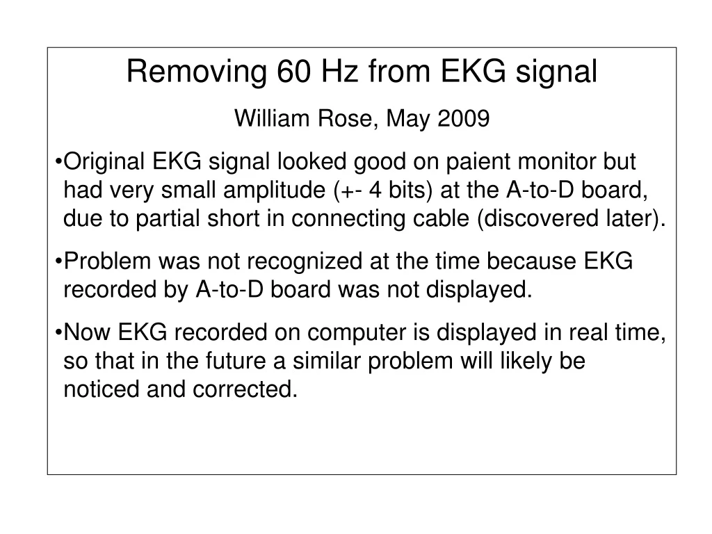
Removing 60 Hz from EKG signal William Rose, May 2009 Original EKG signal looked good on paient monitor but had very small amplitude (+- 4 bits) at the A-to-D board, due to partial short in connecting cable (discovered later).

E N D
Removing 60 Hz from EKG signal William Rose, May 2009 Original EKG signal looked good on paient monitor but had very small amplitude (+- 4 bits) at the A-to-D board, due to partial short in connecting cable (discovered later). Problem was not recognized at the time because EKG recorded by A-to-D board was not displayed. Now EKG recorded on computer is displayed in real time, so that in the future a similar problem will likely be noticed and corrected.
EKG for 10 sec, unfiltered. Noise is large compared to the R waves, preventing triggering. bandstopfilt.vi, 20081111aecg_10sec.txt EKG for 0.5 sec, unfiltered. Notice periodic signal and level quantization due to small amplitude.
Presence of a distinct frequency in the data suggests that a band stop (notch) filter may be useful. • Band stop filters characterized by • Center frequency (Hz) • Bandwidth (Hz) (half width) • Number of poles • Labview and Matlab filter functions want high and low frequencies instead of center frequency and half width.
bandstopfilt.vi • Most code inside a while loop. • Before entering loop: Get file name, read in data, get sampling rate. • Inside the loop, program continually re-filters, re-plots, and checks to see if fco, fhalfwidth, or number of poles have changed. • When while loop is done, program writes data to a file if requested. • Filtering • Butterworth Coefficients.vi • Cascade to Direct Coefficients.vi • Zero Phase Filter.vi • Instead of • (Butterworth Filter.vi, Reverse 1D Array.vi) two times
bandstopfilt.vi Butterworth Coefficients.vi gives filter coefficients in cascade form (2nd order sections for low- and high-pass filters; 4th order sections for band pass and band stop filters). High order filters generally perform better if implemented in cascade form than if implemented in direct form, because they are less sensitive to quantization errors in the coefficients. However, Zero Phase Filter.vi needs direct form. Direct form looks like this: Yk = b0 Xk + b1 Xk-1 + b2 Xk-2 + b3 Xk-3 + b4 Xk-4 + … - a1 Yk-1 –a2 Yk-2 –a3 Yk-3 –a4 Yk-4 – … a’s are the reverse coefficients b’s are the forward coefficients
Front panel of bandstopfilt.vi 20081111aecg_10sec.txt Top: black dots=original, red line=filtered Middle: Power spectrum of original signal. Note logarithmic Y-axis scale and power at 60, 120, 180… Hz. (The 60 Hz noise is not a pure sinusoid, so it has power at harmonics of 60.) Bottom: Power spectrum of filtered signal. Note notch at 60 Hz.
bandstopfilt.vi. • Tests done with input = 20081111aecg_10sec.txt; fcutoff=60 Hz • Change filter width while keeping number of poles fixed: • (fhalfwidth, # poles) = (1 Hz, 4); (5 Hz, 4); (10 Hz, 4). • Change number of poles while keeping width fixed: • (fhalfwidth, # poles) = (10 Hz, 1); (10 Hz, 4); (10 Hz, 8). • Results: “Signal to noise” (size of QRS /size of background noise) changes little, even though power spectrum notches change. • Tests done with white noise input: uniformrandoms.txt; fco=60 Hz • (fhalfwidth, # poles) = (1Hz, 4); (5 Hz, 4); (10 Hz, 4); (10 Hz, 8). • Results: Some combinations resulted in unstable filters, manifested as an output signal which was orders of magnitude too large: (fhalfwidth, # poles) = (5 Hz, 7); (5 Hz, 8); (10 Hz, 8); (10 Hz, 9).
bandstopfilt+harmonics.vi. Add filters at the harmonics: multiples of center frequency. Test with a white noise signal: input=uniformrandoms.txt; fcutoff=60Hz. (fhalfwidth, # poles) = (3 Hz, 1); (5 Hz, 4); (10 Hz, 8). Input = 20081111aecg_10sec.txt; fcutoff=60 Hz. (fhalfwidth, # poles) = (3 Hz, 1); (5 Hz, 4); (10 Hz, 8). “Signal to noise” (size of QRS /size of background noise) is somewhat better with filtering at 60 Hz and its harmonics than with filtering at 60 Hz only.
Comparison of raw signal with output from bandstopfilt.vi and bandstopfilt+harmonics.vi Top: 20081111aecg.txt unfiltered. Middle: bandstopfilt, fco=60 Hz, fhw=5 Hz, order=4 (each way). Bottom: bandstopfilt+harmonics, fco=60 Hz, fhw=5 Hz, order=4 (each way). sample_compare.jpg
bandstopfilt+harmonics+lowpass.vi. Add an optional 4th order Butterworth lowpass filter (forward plus backward to give zero phase) to the bandpass filters. Input = 20081111aecg_10sec.txt fco = 60 Hz, fhw = 20 Hz, order (each way) = 4. flp = 200 Hz “Signal to noise” (size of QRS /size of background noise) is somewhat better with than without the lowpass filter at 200 Hz.