Download
1 / 22
220 likes | 346 Vues
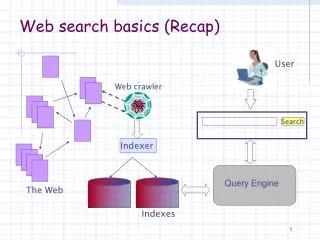
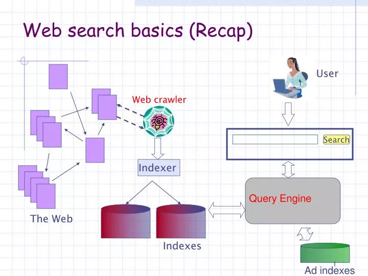
User. Web crawler. Search. Indexer. The Web. Indexes. Ad indexes. Web search basics (Recap). Query Engine. Query Engine’s operations. Process query Look-up the index (and ad indices) Retrieve list of documents (and ads) Order documents Content relevance Link analysis Popularity

E N D
User Web crawler Search Indexer The Web Indexes Ad indexes Web search basics (Recap) Query Engine
Query Engine’s operations • Process query • Look-up the index (and ad indices) • Retrieve list of documents (and ads) • Order documents • Content relevance • Link analysis • Popularity • Prepare results page Today’s question: Given a large list of documents that match a query, how to order them according to their relevance?
Answer: Scoring Documents • Given document d, Given query q • Calculate score(q,d) • Rank documents in decreasing order of score(q,d) • “Bag of words” Model: Documents = bag of [unordered] words (in set theory a bag is a multiset) • John is quicker than Maryand Mary is quicker than Johnhave the same words • A document is composed of terms • A query is composed of terms • score(q,d) will depend on terms
Assign to each term a weight tft,d - term frequency (how often term toccurs in document d) query = ‘who wrote wild boys’ doc1 = ‘Duran Duran sang Wild Boys in 1984.’ doc2 = ‘Wild boys don’t remain forever wild.’ doc3 = ‘Who brought wild flowers?’ doc4 = ‘It was John Krakauer who wrote In to the wild.’ Method 1: Term Frequency tft,d query = {boys: 1, who: 1, wild: 1, wrote: 1} doc1 = {1984: 1, boys: 1, duran: 2, in: 1, sang: 1, wild: 1} doc2 = {boys: 1, don’t: 1, forever: 1, remain: 1, wild: 2} … score(q, doc1) = 1 + 1 = 2 score(q, doc2) = 1 + 2 = 3 score(q,doc3) = 1 + 1 = 2 score(q, doc4) = 1 + 1 + 1 = 3
Why is using just tft,d is not good? • All terms have equal importance. • Bigger documents have more terms, thus the score is larger. • It ignores term order. Postulate: If a word appears in every document, probably it is not that important (it has no discriminatory power).
Sec. 6.2.1 Method 2: Weights according to rarity • Rare terms are more informative than frequent terms • Recall stop words • Consider a term in the query that is rare in the collection (e.g., arachnocentric) • A document containing this term is very likely to be relevant to the query arachnocentric • → We want a high weight for rare terms like arachnocentric. • dft - document frequency for term t • idft - inverse document frequency for term t N - total number of documents
Sec. 6.2.1 idf example, suppose N = 1 million There is one idf value for each term t in a collection.
Effect of idf on ranking • Does idf have an effect on ranking for one-term queries, like • iPhone • idf has no effect on ranking one term queries • idf affects the ranking of documents for queries with at least two terms • For the query capricious person, idf weighting makes occurrences of capricious count for much more in the final document ranking than occurrences of person.
Sec. 6.2.2 Method 3: Better tf-idf weighting • The tf-idf weight of a term is the product of its tf weight and its idf weight. • Best known weighting scheme in information retrieval • Note: the “-” in tf-idf is a hyphen, not a minus sign! • Alternative names: tf.idf, tf x idf • Increases with the number of occurrences within a document • Increases with the rarity of the term in the collection
Sec. 6.2.2 Final ranking of documents for a query
Sec. 6.3 Binary → count → weight matrix Each document is now represented by a real-valued vector of tf-idf weights ∈ R|V|
Sec. 6.3 Documents are vectors • So we have a |V|-dimensional vector space • Terms are axes of the space • Documents are points or vectors in this space • Very high-dimensional: tens of millions of dimensions when you apply this to a web search engine • These are very sparse vectors - most entries are zero. t3 d2 d3 d1 θ φ t1 d5 t2 d4
Sec. 6.3 Queries are also vectors • Key idea 1:Represent queries as vectors in the space • Key idea 2:Rank documents according to their proximity to the query in this space • proximity = similarity of vectors • proximity ≈ inverse of “distance” • Recall: We do this because we want to get away from the you’re-either-in-or-out Boolean model. • Instead: rank more relevant documents higher than less relevant documents
Sec. 6.3 Determine vector space proximity • First cut: distance between two points • ( = distance between the end points of the two vectors) • Euclidean distance? • Euclidean distance is a bad idea . . . • . . . because Euclidean distance is large for vectors of different lengths. t3 d2 d3 d1 θ φ t1 d5 t2 d4
Sec. 6.3 Why Euclidean distance is a bad idea The Euclidean distance between q and d2 is large even though the distribution of terms in the query qand the distribution of terms in the document d2 are very similar.
Sec. 6.3 Use angle instead of distance • Thought experiment: take a document d and append it to itself. Call this document d′. • “Semantically” d and d′ have the same content • The Euclidean distance between the two documents can be quite large • The angle between the two documents is 0, corresponding to maximal similarity. • Key idea: Rank documents according to angle with query.
Sec. 6.3 From angles to cosines • The following two notions are equivalent. • Rank documents in decreasing order of the angle between query and document • Rank documents in increasing order of cosine(query,document) • Cosine is a monotonically decreasing function for the interval [0o, 180o]
Sec. 6.3 Length normalization • A vector can be (length-) normalized by dividing each of its components by its length – for this we use the L2 norm: • Dividing a vector by its L2 norm makes it a unit (length) vector (on surface of unit hypersphere) • Effect on the two documents d and d′ (d appended to itself) from earlier slide: they have identical vectors after length-normalization. • Long and short documents now have comparable weights
Sec. 6.3 cosine(query,document) Dot product Unit vectors qi is the tf-idf weight of term i in the query di is the tf-idf weight of term i in the document cos(q,d) is the cosine similarity of q and d … or, equivalently, the cosine of the angle between q and d.
Sec. 6.3 Cosine similarity amongst 3 documents How similar are the novels SaS: Sense and Sensibility PaP: Pride and Prejudice, and WH: Wuthering Heights? Term frequencies (counts) Note: To simplify this example, we don’t do idf weighting.