Download
1 / 61
680 likes | 931 Vues
Eddy-covariance flux measurements: Outline for the day. Morning ChEAS sites and current research projects Methods (Berger et al, 2001; Yi et al, 2000) Results Published or in press Yi et al 2000, Davis et al, Cook et al. In preparation (with hypotheses) Various, PSU research group members

E N D
Eddy-covariance flux measurements: Outline for the day Morning • ChEAS sites and current research projects • Methods (Berger et al, 2001; Yi et al, 2000) • Results • Published or in press • Yi et al 2000, Davis et al, Cook et al. • In preparation (with hypotheses) • Various, PSU research group members • Future plans/proposals
Eddy-covariance flux measurements:Outline for the day Afternoon • Eddy covariance flux calculation and Li-Cor demo • Small group discussion. Suggested topics: • Causes of interannual variability at WLEF • Causes of differences among ChEAS tower flux measurements • Potential for instrument bias, errors, and improvements • Extension of interannual variability studies beyond ChEAS • Uses of sub-canopy flux and turbulence measurements • Two-dimensional flux experiments and analyses • Caterpillars – observed or imagined?
ChEAS eddy covariance flux measurements I: Sites and research projects
Chequamegon Ecosystem-Atmosphere Study (ChEAS) flux towers WLEF tall tower (447m) CO2 flux measurements at: 30, 122 and 396 m CO2 mixing ratio measurements at: 11, 30, 76, 122, 244 and 396 m Forest stand flux towers: Mature deciduous upland (Willow Creek) Deciduous wetland (Lost Creek) Mixed old growth (Sylvania) All have both CO2 flux and high precision mixing ratio measurements.
North Upland, wetland, and very tall flux tower. Old growth tower to the NE. High-precision CO2 profile at each site. Mini-mesonet, 15-20km spacing between towers. Lost Creek Landcover key Open water WLEF Wetland Coniferous Mixed deciduous/coniferous Shrubland Willow Creek General Agriculture
ChEAS web sites • http://cheas.psu.edu - Main page. • ftp://ftp.essc.psu.edu/pub/workgroup/davis/ - Data access. • http://cheas.psu.edu/fieldsites.html - Site descriptions. Also see: • http://www.daac.ornl.gov/FLUXNET/fluxnet.html - Fluxnet’s home page, and, • http://public.ornl.gov/ameriflux/Participants/Sites/Map/index.cfm - AmeriFlux’s home page.
Research Funding • Regional atmosphere/forest exchange and concentrations of carbon dioxide. • Study of net ecosystem exchange of carbon dioxide via eddy covariance measurements at the WLEF tower in northern Wisconsin, as well as the study of carbon dioxide transport and distribution within the boundary layer. • PI: P.S. Bakwin, U. Colorado/NOAA • Co-I: K.J. Davis Penn State • Department of Energy, National Institutes for Global Environmental Change • Duration: July, 1994–June, 1997; July, 1997–June, 2000; July, 2000–June 2003. • Measuring and modeling component and whole-system CO2 fluxes at local to regional scales. • Study of component processes which make up CO2 fluxes in a forest ecosystem, and comparison to whole-ecosystem net flux measurements from small flux towers. Also a comparison between homogeneous ecosystem fluxes within the WLEF tower footprint and the WLEF net flux signal. • PI: P.V. Bolstad, U. Minnesota • Co-Is: K.J. Davis, Penn State, and P.B. Reich, U. Minnesota • Department of Energy, National Institutes for Global Environmental Change • Duration: July, 1997 - June, 2000. July 2000 – June 2003.
Research Funding • Quantifying carbon sequestration potential of mid and late successional forests in the upper Midwest • Observations of CO2 exchanges in an old-growth forest in the upper peninsula of Michigan and comparison to existing flux towers in younger forest stands northern Wisconsin. Davis's work would provide tower construction, instrumentation, and data analysis support for a 30m tower. • PI: Eileen Carey, U. Minnesota • Co-Is: P.V. Bolstad, U. Minnesota; K.J. Davis, Penn State • Department of Energy, Terrestrial Carbon Processes • Duration: January, 2001 - December, 2003 • Regional forest-ABL coupling: Influence on CO2 and climate • Study of the coupling between the surface energy balance, boundary layer development, and net ecosystem exchanges of carbon dioxide, as well as the influence of the covariance between carbon dioxide fluxes and boundary layer development on boundary layer mixing ratios of carbon dioxide. Observations at the WLEF and the Walker Branch AmeriFlux sites using an NCAR radar. • PI: K.J. Davis, Penn State • Co-I: A.S. Denning, Colorado State University • Department of Energy, TECO/Terrestrial Carbon Program • Duration: September, 1997 - August, 2002
ChEAS eddy covariance flux measurements II: Methods
Methods: Eddy covariance flux measurements in ChEAS • Basic theory of eddy covariance flux measurements. • Tower flux instrumentation • LI-COR calibration • Sonic rotation • Lag time correction • Spectral corrections • Random and systematic errors due to turbulence • “Preferred” NEE algorithm (WLEF only) • Filling missing data
Publications describing methodology • Yi, C., K.J. Davis, P.S. Bakwin, B.W. Berger, and L. C. Marr, 2000. The influence of advection on measurements of the net ecosystem-atmosphere exchange of CO2 observed from a very tall tower,J. Geophys. Res. 105, 9991-9999. • Berger, B.W., K.J. Davis, P.S. Bakwin, C. Yi and C. Zhao, 2001. Long-term carbon dioxide fluxes from a very tall tower in a northern forest: Flux measurement methodology. J. Atmos. Oceanic Tech., 18, 529-542. • Davis, K.J., P.S. Bakwin, B.W. Berger, C. Yi, C. Zhao, R.M. Teclaw and J.G. Isebrands, The annual cycles of CO2 and H2O exchange over a northern mixed forest as observed from a very tall tower. Global Change Biology, in press.
Theory “Reynold’s averaged” (= mean + turbulent components of all variables) scalar conservation equation. Time rate of change (e.g. CO2) Mean transport Turbulent transport (flux) Source in the atmosphere Integrate from the earth’s surface to the imaginary plane defined by the level of the flux sensor.
Theory Yi et al, 2000
Theory: What is w’c’? • Prime indicates departure from the mean. • w’ > 0 is an updraft • c’ > 0 is air rich in the scalar c • w’c’ > 0 is upwards transport of the scalar • Averaging this over time sums the transport observed due to all updrafts and downdrafts.
Daily cycle of ABL depth, and CO2 fluxes and mixing ratios Radar ABL depth WLEF fluxes CO2 profile Davis et al, in press
Diurnal cycle of CO2 in the ABL Bakwin et al, 1998
Instruments at WLEF Berger et al, 2001
Instruments at WLEF • Two “profiling” LI-CORs in the trailer, one sampling 396m, one cycling among all 6 levels. “Slow” time response. High-precision and accuracy calibration (Bakwin et al, 1998). C-bar. • Vaisala humidity and temperature sensors at 3 levels (30, 122 and 396m). “Slow” Q-bar, T-bar. • Three sonic anemometers (30, 122 and 396m). w’, T’ • Three LI-CORs in the trailer, one for each sonic level. “Fast” time response. Long tubes, big pumps. Measure CO2 and H2O. c’, q’ • Two LI-CORs on the tower (122 and 396m). “Fast” time response. Short tubes, smaller pumps.
Calibration of “fast” CO2 and H2O sensors at ChEAS towers • Calibration occurs using the fluctuations in the ambient atmospheric CO2 and H2O mixing ratios. • “Slow” sensors provide absolute values of these mixing ratios used to calibrate the “fast” LI-CORs. • Ideal gas law corrections to LI-COR cell temperature, pressure and humidity are applied. • Calibration slope and intercept are derived every 2 days. These values are smoothed (monthly running mean) to derive the long-term calibration factors used for the “fast” LI-CORs.
Calibration of “fast” CO2 and H2O sensors Berger et al, 2001
What’s up? (Sonic rotations) • Sonic anemometers are oriented perfectly in the vertical, (and the wind’s “streamlines” aren’t always perpendicular to gravity). • Data is collected over a long time (about a year) and we define “up” by forcing the mean vertical wind speed to be zero.
Sonic rotations Berger et al, 2001
Lag time calculation • We must correct for the delay between the CO2 and H2O measurements and the vertical velocity measurements. • Lag time is determined by finding the maximum in the lagged covariance between vertical velocity and CO2/H2O for every hour. Berger et al, 2001
Lag time calculation Berger et al, 2001
Spectral corrections • Flow through tubes smears out some of the atmospheric fluctuations, especially the small (high frequency) eddies. • Obvious for H2O. Much worse than theory predicts. • Not directly observed for CO2. Small effect. • The sonic anemometer (virtual) temperature measurement is not smeared out, so we use similarity between the virtual temperature spectrum and the water vapor spectrum to correct for the loss of high frequency eddies in H2O. • We use past studies of flow in tubes to correct for the loss of high frequency eddies in CO2.
Spectral corrections CO2 Berger et al, 2001 Tv H2O
Spectral corrections Table shows the typical % of flux lost due to smearing of small eddies. Berger et al, 2001
Systematic errors – getting the large and small eddies Berger et al, 2001
Random errors – a finite number of eddies are counted in one hour Random sampling errors for any one hour can be as large as the magnitude of the measured flux! Berger et al, 2001, following Lenschow and Stankov, 1986.
“Preferred” NEE (WLEF only) • Data is taken from 30m at night and 122 or 396m during the day (the highest level where there is turbulent flow) when all data are available. • If data are missing, any existing flux measurement is used. • Data are screened out when the level of turbulence is very low. CO2 is probably draining down hill. • Early in the morning upper level data from WLEF is replaced with 30m data (Yi et al, 2000) because the flow appears to be systematically 2-D. • Thus from 3 NEE measurements, one is derived as our “preferred” measurement for each hour.
Nighttime drainage flows? Loss of flux at low turbulence levels at the Willow Creek tower. Cook et al, submitted; Davis et al, in press
Morning advection at WLEF Yi et al, 2000
Multiple level comparison at WLEF Davis et al, in press Comparison of all 3 levels, growing season 1997.
ChEAS eddy covariance flux measurements III: Results
Missing data, gross fluxes, light and temperature response • Nighttime NEE measurements (for CO2) are fitted to soil or air temperature. This is assumed to describe the total respiration flux. • Daytime NEE measurements are fitted to PAR after total respiration has been computed using the fits and “subtracted” from NEE. This fit describes the response of forest photosynthesis to sunlight. • These fits are used to compute gross fluxes (respiration, photosynthesis) and to fill in missing NEE data needed to compute cumulative NEE.
Gross fluxes and functional fits Davis et al, in press
Example of gross fluxes fit to temperature and PAR at WLEF for one month. Davis et al, in Press.
Hourly fluxes at WLEF for 1997, observed and filled. Davis et al, in press.
Cumulative fluxes at WLEF, 1997 Davis et al, in press
Gross fluxes at WLEF, 1997 RE Davis et al, in press NEE -GEP
Method NEE GEP RE Low U* screened, T-PAR fill 16 +/- 19 947 963 Low U* retained -48 +/- 20 864 816 Low U* screened, median fill -25 +/- 17 891 867 1997 Cumulative NEE, GEP and RE vs. assumptions and methods (gC m-2 yr-1 = tC ha-1 yr-1 * 100) Davis et al, in press
Lack of energy balance: Are turbulent fluxes underestimated? Davis et al, in press Cook et al, submitted
Monthly mean CO2 fluxes at WLEF, 1997. Davis et al, in press
Monthly mean latent heat fluxes at WLEF, 1997. Davis et al, in press
Bowen ratio vs. time of year at WLEF, 1997. Davis et al, in press, following Cook et al, submitted.


![EDT1-EDDY Center [mg/m -2 /day -1 ] Depth Mass C-Flux N-Flux](https://cdn2.slideserve.com/4289367/slide1-dt.jpg)