Download
1 / 33
410 likes | 606 Vues
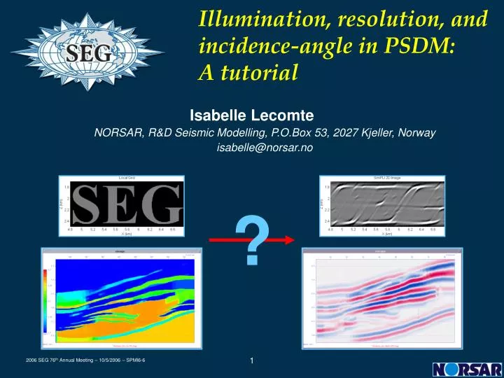
?. Illumination, resolution, and incidence-angle in PSDM: A tutorial. Isabelle Lecomte NORSAR, R&D Seismic Modelling, P.O.Box 53, 2027 Kjeller, Norway isabelle@norsar.no. Space-variant PSF!. Hubble telescope: space-variant PSF*. *Point-Spread Functions. http://huey.jpl.nasa.gov/mprl.

E N D
? Illumination, resolution, and incidence-angle in PSDM:A tutorial • Isabelle Lecomte • NORSAR, R&D Seismic Modelling, P.O.Box 53, 2027 Kjeller, Norway • isabelle@norsar.no
Space-variant PSF! Hubble telescope: space-variant PSF* *Point-Spread Functions http://huey.jpl.nasa.gov/mprl
Seismics: PSF may be very space-variant! Point-Spread Functions in Marmousi* *Marmousi model courtesy of IFP
* ** Acoustic/elastic impedance Reflection ~ contrasts! PSDM … at best! Not 1D convolution! ! Resolution, illumination, …etc! *http://www.lenna.org , **Liner (2000), and Monk (2002)
Content • Introduction • Image formation in PSDM • Scattering wavenumber: the key! • Resolution • Illumination • Examples • Controlling imaging • Conclusions
Migration (*)GF: Green’s Function Waves! Waves! Key information: Scattering Wavenumber! Back propagation 1 G,G:GF(*) ●: GF-node Incident wave Wave propagation corrections Waves! Imaging ? 2 Imaging Scattering Focusing Imaging in PSDM: K is the key! Getting data
Model: constant velocity Data: point scatterer ■ ■ Common shot (x = 0) Common offset (0 m) data data ■ ● point scatterer ellipse circle PSDM PSDM Scattering isochrones
■ ■ ■ ■ ■ ■ ■ ■ ■ ■ ■ ■ ■ ■ ■ ■ Same point scatterer… ● ● ● ● ● ● ● ● ● ● ● ● ● ● ● ● …different PSDM images! PSDM and point scatterer Common offset (0 m) 1 trace ∑ traces Common shot (x = 0) ■ ■ ■ ■ ■ ■ ■ ■ ■ ■ ■ ■ ■ ■ ■ ■ ● 1 trace ∑ traces
PSF and PSDM: why? • scattering structures = set of point scatterers (e.g., exploding reflector concept, etc) • PSDM(point scatterer) = Point-Spread Function • If PSF known: PSDM image = Reflectivity * PSF • Question 1: how to get PSF without generating synthetic point scatterers at each image point? • Question 2: how to use PSF to understand and improve PSDM?
Content • Introduction • Image formation in PSDM • Scattering wavenumber: the key! • Resolution • Illumination • Examples • Controlling imaging • Conclusions
● (*) patent pending Methods: ”ray-tracing” based • Green’s functions • Paraxial ray tracing • Wavefront Construction • Eikonal solver • PSDM(~Kirchhoff) • Diffraction Stack (DS) • Local Imaging (LI) • 1 GF-node only! • ”SimPLI” (*) • Simulated Prestack Local Imaging • No seismic records needed!
Incident wavenumber scattered wavenumber Scattering Wavenumber K Definition at a local “Scattering Object” (diffraction, reflection, ..) Easy to calculate with ray tracing and similar Calculation performed in the PSDM velocity model
geophone g source s • - Vs: incident wave velocity • Vg: scattered wave velocity • ŝ and ĝ: unit vectors • n frequency • - VP: P-velocity • VS: S-velocity K If Vs = Vg (no wave conversion) K ŝ ŝ ĝ ĝ ● ● ● ”incidence” angle = 0 ║ĝ – ŝ║ = 2 ”incidence” angle ≠ 0 ║ĝ – ŝ║ < 2 K: which parameters?
X no data! -Kx max. +Kx max. PSF -Kz max. Green’s Functions at one GF-node max./2 2D FFT-1 Z module ● 0 ● 0. ● 2D FFT Marmousi ● From K to PSF using FFT
K is perpendicular to the scattering isochrone ║K ║ = f(n) : pulse effect K corresponds to a local plane wavefront approximation of the scattering isochrone [K] PSF K and scattering isochrones
Content • Introduction • Image formation in PSDM • Scattering wavenumber: the key! • Resolution • Illumination • Examples • Controlling imaging • Conclusions
Your model! Generalized Inverse 1 2 Direct problem Inverse problem Resolution! 1+2 Data independent! Resolution of an inverse problem! d: data m: parameters obs.: observed est.: estimated
[K]for [5-60] Hz qs = [0-10] º DKZ DKx 1 Lateral resolution ~ 2p / DKX Vertical resolution ~ 2p / DKZ K and resolution: wavenumber coverage Marmousi model Courtesy of IFP
K Kmean low R high R PSF K and PSF: no data! K Kmean high R low R PSF PSDM of point scatterer and PSF Common offset (0 m) PSDM – data from point scatterer Common shot (x = 0)
Content • Introduction • Image formation in PSDM • Scattering wavenumber: the key! • Resolution • Illumination • Examples • Controlling imaging • Conclusions
From source To geophone From source To geophone qs qg qs qg incident ray reflected ray qs incidence angle qgscattering angle K and reflection ”P-to-P” reflection ”P-to-S” reflection Reflector Reflector • In the PSDM velocity model: • A given couple (ks,kg) may correspond to an actual reflection. • it is the case IF there is a reflector perpendicular to K at the GF-node.
[K]for [5-60] Hz qs = [0-10] º 2 Illuminated dips ~ 25 º ~ 45 º K and illumination: dip Marmousi model Courtesy of IFP Marmousi Model Courtesy of IFP
Content • Introduction • Image formation in PSDM • Scattering wavenumber: the key! • Resolution • Illumination • Examples • Controlling imaging • Conclusions
120 Hz [K] Target model (Vp) Reflectivity 0 Hz Spectrum 10 Hz 20 Hz 30 Hz 40 Hz SimPLI SimPLI SimPLI SimPLI Playing with the pulse
Fault “Green’s Functions” Reflectivity = 1 [K] incl. 20 Hz pulse Fault Fault PSF SimPLI – 0 km offset 0 km offset FFT-1 FFT-1 FFT+1 FFT-1 FFT-1 Fault Fault PSF 4 km offset SimPLI – 4 km offset Illumination and resolution: illustration
Σ Final SimPLI Image – 20 Hz Incidence-angle in PSDM Reflectivity : 00°-05° Reflectivity : 05°-15° Reflectivity : 15°-25° Reflectivity: 35°-45° Reflectivity: 25°-35° [K] Filter : 15°-25° [K] Filter : 25°-35° [K] Filter : 00°-05° [K] Filter : 05°-15° [K] Filter: 35°-45° SimPLI Image: 00°-05° SimPLI Image: 15°-25° SimPLI Image: 25°-35° SimPLI Image: 35°-45° SimPLI Image: 05°-15°
A B ● ● Not illuminated! Good resolution Good illumination Poor resolution Bad illumination K PSF K PSF Overburden effects
KX KX KX This is PSDM effects! No illumination effects! KZ KZ KZ Elastic impedance (x,z) “1D” PSDM 2D Filter: 0 km offset 2D Filter: 4 km offset ! Function of survey, overburden, pulse, wave-phases, local velocity. PSDM images: not a simple 1D convolution!
Content • Introduction • Image formation in PSDM • Scattering wavenumber: the key! • Resolution • Illumination • Examples • Controlling imaging • Conclusions
Dshot: 12.5 m Dshot: 125 m Dshot: 625 m K K K PSF PSF PSF SimPLI SimPLI SimPLI Image and survey sampling
Blind! Controlled! Controlling imaging: check local K! ”blind!” automatic corrections Irregular Sampling!
Conclusions • Define your PSDM velocity model… • Should be smooth in the imaging zone… • … but can have layers with contrast outside! • …then use the scattering wavenumbers! • Prior or after imaging • Survey planning mode • Resolution/illumination analyses • Controlling and improving imaging • Understanding image formation • Testing the validity of interpretation results • Flexible and fast! • Ray tracing based • FFT
Acknowledgements • Research Council of Norway (projects 131341/420, 128440/43, and 153889/420) • Statoil (Gullfaks), IFP (Marmousi), Seismic Unix, and the “Svalex” project (www.svalex.net, Storvola) • Håvar Gjøystdal, Åsmund Drottning and Ludovic Pochon-Guerin. • Thanks