Download
1 / 31
310 likes | 429 Vues
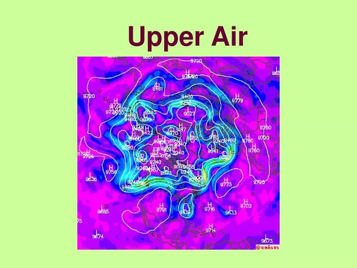
Upper Air. Using just the surface is like diagnosing a sick person using only an examination of the soles of the feet. The atmosphere is three-dimensional. And important stuff (like the jet stream shown here) are not seen directly on a surface map.

E N D
Using just the surface is like diagnosing a sick person using only an examination of the soles of the feet.
The atmosphere is three-dimensional And important stuff (like the jet stream shown here) are not seen directly on a surface map.
3-D views are amazing, but almost all analysis is done using 2-D map views of upper air pressure surfaces.
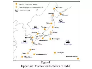
The upper air network is much more sparse than at the surface. Data also can be input via aircraft observations or special radiosondes.
While the U.S. radiosonde station network looked a bit thin, it is much better than most of the world. Only Europe has a comparable density of stations.
Here’s an interesting case: the Valentine’s Day storm of 2007 As we will learn later in the course, 983 mb is deep, but not spectacularly intense for a coastal cyclone.
However, some of these snow totals were spectacular. Oneonta’s 30 inches set the record. This storm had more features than just the surface Low.
At 850 mb, the storm center is over the Chesapeake Bay (remember where it was at the surface?) All pressures are 850 mb and the height of the surface (above sea level) is reported in decameters (dm). Temperatures are in Celsius degrees. The black lines are isoheights (contours), not isobars. Isotherms are colored.
Here’s a closeup of the storm at 850 mb. A more modern unit for a millibar is called a hectopascal, hPa. So this is the 850 hPa surface. What is happening over New York? Use all the information shown.
At 700 hPa, the closed low is hardly there, but the trough covers half the continent. 700 hPa is around (~) 300 dm (~10000 feet)
No closed Low here! 500 hPa is around half the atmosphere. It tends to be at 550 dm (~18000 ft)
Upper air maps are at standard or mandatory levels. The next level up from 500 hPa is 300 hPa. At 300hPa, RH is no longer an important factor. Wind speed is. The maximum observed wind is 140 knots (161 mph) at LCH. But that isn’t the maximum wind in the system.
At 250 hPa the max windspeed is probably over 150 kt (172.5 mph). This level is near the tropopause.
200 hPa heights are well over 1100 dm (35750 ft) and are in the stratosphere. Notice the trough pattern is almost identical from 500 hPa on up.
Thickness is a concept often used with upper air maps. It is simply the difference in heights between two constant height surfaces. The most commonly used value is the 1000-500 mb thickness. The red and blue dashed lines are the values of 1000-500 mb thickness
Derivation of the hypsometric formula Start with the equation of state and the hydrostatic formula: P = ρRT or ρ = P/RT ∂P/∂Z = - ρg Since ρ is common to both, replace it in the hydrostatic formula: ∂P/∂Z =- Pg/RT Move the P to the left side and divide the derivative: ∂P/P = - g∂Z/RT The definition of the natural logarithm means the left side is: ∂(ln P) = - g∂Z/RT
On the right, g and R are constants but T depends on Z: ∫∂(ln P) = - g/R ∫∂Z/T (we will want to integrate from level 0 to level 1) Furthermore, we don’t know the functional form for T with Z. That’s a sounding and, on any individual day, it is unique. For example, the red line shown here is the function T with increasing Z (decreasing P):
Our solution: Use an approximate value for T which is constant with increasing Z. Call it T. Then T can be taken outside the integral: ∫∂(ln P) = - g/RT ∫∂Z Integrate lnP from Po to P1 and Z from Zo to Z1: lnP1 – lnPo = -g/RT(Z1-Zo) Multiply both sides by -1 to get rid of the negative sign: lnPo – lnP1 = g/RT(Z1-Zo) Mathematically, subtracting logarithms is the same as dividing them: ln(Po/P1) = g/RT(Z1-Zo)
The difference between levels, Z1-Zo is the thickness of the layer from P1 to P0: So, ln(Po/P1) = g/RT∆Z Other than constants, Finally, ∆Z = (RT/g) ln(Po/P1) the thickness depends on the mean temperature of the layer! We often take the levels to be 1000 hPa and 500 hPa, but any two levels can be used.
Example: What is the 1000-500 mb thickness if the mean temperature is -7C? R = 287 m2 s-2 k-1, g = 9.8 m s-2, T = -7C = 266K, P0 = 1000 hPa, P1 = 500 hPa ∆Z = (RT/g) ln(Po/P1) ∆Z = (287 m2 s-2 k-1 x 266K/9.8 m s-2) ln 2 ∆Z = 5399.6 m which is approximately 540 decameters (540 dm)
In typical situations when the mean temperature is -7C, the surface is at or close to 0C. This is often the deciding factor between rain and snow. Here the 500 hPa temperature is -16C so the lapse rate is ~ 3C/km)
For places near sea level, the rain/snow line is where the thickness lines change color, at 540 dm.
Radar showed heavy precipitation in central NY and eastern PA, but also in NJ and in NYC.
South of the 540 dm thickness, the snowfall amounts drop off dramatically. Probably most of their precipitation was rain, with a few inches at the end of the storm as the cold air moved in.
How about a tropical situation? What does the upper air look like?