Download
1 / 66
690 likes | 876 Vues
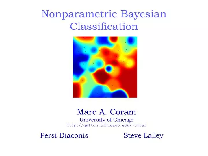
Nonparametric Bayesian Classification. Marc A. Coram University of Chicago http://galton.uchicago.edu/~coram. Persi Diaconis Steve Lalley. Related Approaches. Chipman, George, McCullough Bayesian CART (1998 a,b) Nested CART-like Coordinate aligned splits Good “search” ability

E N D
Nonparametric Bayesian Classification Marc A. Coram University of Chicago http://galton.uchicago.edu/~coram Persi Diaconis Steve Lalley
Related Approaches • Chipman, George, McCullough • Bayesian CART (1998 a,b) • Nested • CART-like • Coordinate aligned splits • Good “search” ability • Denison, Mallick, Smith • Bayesian CART • Bayesian splines and “MARS”
Outline • Medical example • Theoretical framework • Bayesian proposal • Implementation • Simulation experiments • Theoretical results • Extensions to a general setting
Example: AIDS Data(1-dimensional) • AIDS patients • Covariate of interest: viral resistance level in blood sample • Goal: estimate conditional probability of response
Idealized Setting (X,Y)iid pairs X (covariate)X [0,1] Y(response) Y {0,1} f0(true parameter)f0(x)=P(Y=1|X=x) What, then, is a straightforward way to proceed, thinking like a Bayesian?
Prior on f: 1-dimension • Pick a non-negative integer M at randomSay, choose M=0 with prob 1/2 M=1 with prob 1/4 M=2 with prob 1/8 …. • Conditional on M=m, Randomly choose a step function from [0,1] into [0,1] with m jumps • (i.e. locate the m jumps and (m+1) valuesindependently and uniformly)
Perspective • Simple prior on stepwise functions • Functions are parameterized by: • Goal: Get samples from the posterior; average to estimate posterior mean curve • Idea: Use MCMC, but prefer analytical calculations whenever possible # regions jump locations function values
Observations • The joint distribution of U, V, and the data has density proportional to: • Conditional on u, the counts are sufficient for v. where:
Observations II The marginal of the posterior on U has density proportional to: Where: Conditional on U=u and the data, V’s are independent Beta random variables and
Consequently… • In principle: • We put a prior on piecewise constant curves • The curves are specified by • u, a vector in [0,1]m • v, a vector in [0,1]m+1 • for some m • We sample curves from the posterior using MCMC • We take the posterior mean (pointwise) of the sampled curves • In practice: • We need only sample from the posterior on u • We can then compute the conditional mean of all the curves with this u.
Implementation • Build a reversible base chain to sample U from the prior • E.g., start with an empty vector and add, delete, and move coordinates randomly • Apply Metropolis-Hastings to construct a new chain which samples from the posterior on U • Compute:
Simulation Experiment (a) n=1024 • True • Posterior Mean
n=1024 • True • Posterior Mean
n=1024 • True • Posterior Mean
n=1024 • True • Posterior Mean
Classification and Regression Trees(CART) • Consider splitting the data into the set with X<x and the set with X>x • Choose x to maximize the fit • Recurse on each subset • “Prune” away splits according to a complexity criterion whose parameter is determined by cross-validation • Splits that do not “explain” enough variability get pruned off
Simulation Experiment (b) • True • Posterior Mean • CART
Bagging • To “bag” an estimator you treat the estimator as a black box • Repeatedly, generate bootstrap resamples from the data set and run the estimator on these new “data sets.” • Average the resulting estimates
Simulation Experiment (c) • True • Posterior Mean • CART • Bagged Cart: Full Trees
Simulation Experiment (d) • True • Posterior Mean • CART • Bagged Cart: cp=0.005
Simulation Experiment (e) • True • Posterior Mean • CART • Bagged Cart: cp=0.01
CART Bagged CART: cp=0.01
Bayesian Consistency • Consistent at f0 if: The posterior probability of N tends to 1 a.s. for any > 0 • Since all f are bounded in L1, Consistency implies a fortiori that:
Related WorkDiaconis and Freedman (1995) DF: K~ Given K=k, split into 2kequal pieces. (k=3) • Similar hierarchical prior, but: • Aggressive splitting • Fixed split points • Strong Results: • If dies off at a specific geometric rate • Consistency for all f0 • If dies off just slower than this • Posterior will be inconsistent at f0=1/2 • Consistency results cannot be taken for granted
Consistency Theorem: Thesis If(Xi,Yi) are drawn iid via (i=1..n) X ~ U(0,1) Y|X=x ~ Bernoulli(f0(x)) And if is the specified prior on f, chosen so that the tails the prior on hierarchy level M, decay like exp(-n log(n) ) Thenn, the posterior, is a consistent estimate of f0, for any measurable f0.
Method of Proof • Barron, Schervish, Wasserman (1999) • Need to show: • Lemma 1: Prior puts positive mass on all Kullback-Leibler information neighborhoods of f0 • Choose sieves: Fn={f: f has no more than n/log(n) splits} • Lemma 2: The -upper metric entropy of Fnis o(n) • Lemma 3: (Fnc) decays exponentially
New Result • Coram and Lalley 2004/5 ( hopefully ) • Consistency holds for any prior with infinite support, if the true function is not identically ½. • Consistency for the ½ case depends on the tail decay* • Proof revolves around a large-deviation question: • How does predictive probability behave as n --> infinityfor a model with m=an splits? (0<a<infinity) • Proof uses subadditive ergodic theorem to take advantage of self-similarity in the problem
Flip a fair coin repeatedly 1/2 1/2 Pick p in [0,1] at random Flip that p-coin repeatedly A Guessing Game
A Voronoi Prior for [0,1]d 1 2 V1 V2 V3 5 V5 3 V4 4
A Modified Voronoi Prior for General Spaces • Choose M, as before • Draw V=(V1, V2, … Vk) • With each Vj drawn without replacement from an a-priori fixed set A • In practice, I take A={X1, …, Xn} • This approximates drawing the V’s from the marginal dist of X
Discussion • CON: • Not quite Bayesian • A depends on the data • PRO: • Only partitions the relevant subspace • Applies in general metric spaces • Only depends on D, the pairwise distance matrix • Intuitive Content