Download

1 / 33
330 likes | 442 Vues
Connectivity in SoCal Bight. UCLA-UCSB Telecon 1/14/08. Lagrangian Particle Tracking. Used 6-hourly mean flow fields from 1996 thru 1999 (Thanks, Charles!) 1-hour time stepping for particle tracking Output particle data every 6 hours Used UCLA particle tracking code

E N D
Connectivity in SoCal Bight • UCLA-UCSB Telecon 1/14/08
Lagrangian Particle Tracking • Used 6-hourly mean flow fields from 1996 thru 1999 • (Thanks, Charles!) • 1-hour time stepping for particle tracking • Output particle data every 6 hours • Used UCLA particle tracking code • Released within 10 km from coast • Every 1 km, every 6 hours (32,748 particles / day) • Depth is fixed at 5 m below top surface
Single-day, Single-point Release(30-day trajectories) Release = Jan 1, 1996 Release = Jan 1, 1997 Red dots = location 30 days later Release location Release = Jan 1, 1998 Release = Jan 1, 1999 • Particles released on the same date from the same location show different dispersal patterns every year
Single-day, Single-point Release(30-day trajectories) Release = Jan 1, 1996 Release = Jan 16, 1996 Red dots = location 30 days later Release location Release = Jan 31, 1996 Release = Feb 15, 1999 • 2 weeks of difference in release timing can result in very different dispersal patterns
Single-day, Single-Point Release(30-day trajectories) Near San Diego Palos Verdes Release location • Dispersal patterns depend on release locations
Points • Dispersal patterns show strong intra- & inter-annual variability (turbulent dispersion) • Particles released at the same location on the same day shows different patterns every year • 15 days of difference in release timing can lead to different dispersal patterns • Dispersal patterns depend on release location • Trajectories show chaotic eddying motions, very different from a simple diffusion process • We need statistical description
Comparison with Drifter Data (Not done yet. Hopefully done by Monday)
Lagrangian (Transition) PDF • Probability density of Lagrangian particle location after time interval tau from release • Estimate using all particles (1996-1999) • First, we neglect inter- & intra-annual variability • Pretend as if they were statistically stationary processes (i.e., independent of t0) and assume ergodicity... Particle location after time interval tau Particle release location & date
Lagrangian (Transition) PDF x0 = San Nicholas Island tau = 1 day tau = 10 days Release location tau = 20 days tau = 30 days • Spread out in 20-30 days; more isotropic (Bin size: 5 km radius in space; 1 day in time)
Lagrangian (Transition) PDF x0 = Near San Diego (Oceanside) tau = 1 day tau = 10 days Release location tau = 20 days tau = 30 days • Strong directionality (pole-ward transport) (Bin size: 5 km radius in space; 1 day in time)
From 9 Different Sites tau = 30 days pole-ward transport eddy retention Release location more isotropic spread • Strong release-position dependence
Connectivity Matrix • Lagrangian PDF in a matrix form • Or, we can average Lagrangian PDF over some time interval (larval fish dispersal case) (We can do weighted-mean, too)
Site Locations & Connectivity S. Islands N. Islands Mainland Mainland N. Islands S. Islands • Pole-ward transport & eddy retention show up in connectivity
As a Function of Evaluation Time tau = 30 days tau = 35 days tau = 40 days tau = 45 days tau = 20 -- 40 days tau = 24 -- 48 days tau = 28 -- 56 days tau = 32 -- 64 days • Spatial structures in connectivity fade away as tau increases (well mixed) • Time averaging does not change connectivity
Source & Destination Strength • Summation of connectivity matrix over i or j (Would be useful for MPA design)
Source & Destination Strength tau = 30 days tau = 30 days tau = 40 days tau = 40 days • Strongest Destination at Chinese Harbor • Match well with observation (not shown here)
Summary • Lagrangian particle can reach entire Bight in 30 days • Dispersal patterns show release-position dependence • Strong directionality along mainland • More isotropic from Islands • Eddy retention in Channel & near San Clemente Island • After spreading out in entire Bight, spatial patterns in Lagrangian PDF gradually fade away • Particles either go out of domain or go any places in Bight (well mixed)
Summary • Connectivity shows spatial patterns, reflecting pole-ward transport along mainland & eddy retention • But, spatial patterns fade away in time (~ 60 days) • As particles from various sources become well mixed • Almost all sites can be connected in 30 days • Source & destination strength patterns: • Strong source: mainland (SD ~ SB) • Strong destination: Santa Cruz, E. Anacappa, E. San Nicolas, North mainland (Palos Verdes ~ SB) • Strongest destination: Chinese Harbor (self retention + transport from mainland)
Inter-annual Variability • Compute Lagrangian PDF using particles released in a particular year instead of using all years • 1) 1996, 2) 1997, 3) 1998, or 4) 1998 • Let’s see PDF shows inter-annual variability
Lagrangian (Transition) PDF x0 = Near San Diego (Oceanside), tau = 30 days Release location • Alongshore transport disappears in 1999 (La Nina); very strong in 1997 (El Nino) • Important for species invasion from Mexico
Lagrangian (Transition) PDF x0 = north shore of Santa Cruz Island, tau = 30 days Release location • Eddy retention does not occur every year • Important for species retention
Destination Strength tau = 30 days
Source Strength tau = 30 days
Summary • Lagrangian PDF shows strong inter-annual variability • Northward transport is strongest in 1997 (El Nino), while it disappears in 1999 (La Nina). • Eddy retention does not appear every year • These will mean a lot to population ecology • Source & destination strength changes accordingly
Seasonal Variability • Compute Lagrangian PDF using particles released in a particular season • 1) Winter of 1996-1999, • 2) Spring of 1996-1999, • 3) Summer of 1996-1999, and • 4) Autumn of 1996-1999 • Seasonal variations are expected
Lagrangian (Transition) PDF x0 = Near San Diego (Oceanside), tau = 30 days Release location • Pole-ward transport disappears spring & summer when equator-ward wind is strong
Lagrangian (Transition) PDF x0 = north shore of Santa Cruz Island, tau = 30 days Release location • Eddy retention is weakened in spring & summer when equator-ward wind is strong
Lagrangian (Transition) PDF x0 = Palos Verdes Peninsula, tau = 30 days Release location • Palos Verdes shows self retention in summer possibly due to wind sheltering
Inter-annual & Seasonal Variability in Connectivity tau = 30 days Self retention at many sites Self retention at limited sites Pole-ward transport • Seasonal variability is stronger than inter-annual variability (as expected)
Source Strength tau = 30 days
Destination Strength tau = 30 days
Summary • Lagrangian PDF shows strong inter-seasonal variability (as expected) • Pole-ward transport along the mainland appears fall & winter; gone in spring & summer • Eddy retention in Channel appears fall & winter • Depending on strength of equator-ward wind • Seasonal patterns in connectivity are: • Winter: strong self retention at many sites • Spring & summer: strong self retention at limited places • Fall: strong pole-ward transport
Applications (to be done) • We need several applications here • Ex. 1. Dispersal of fish larvae • Ex. 2. Spread of pollutants • Given distributions of materials at x0 and t0, concentrations of materials after tau are given by This can be larval production, oil spill distributions & etc If molecular diffusion & chemical reactions are negligible, though