Download
1 / 31
330 likes | 606 Vues
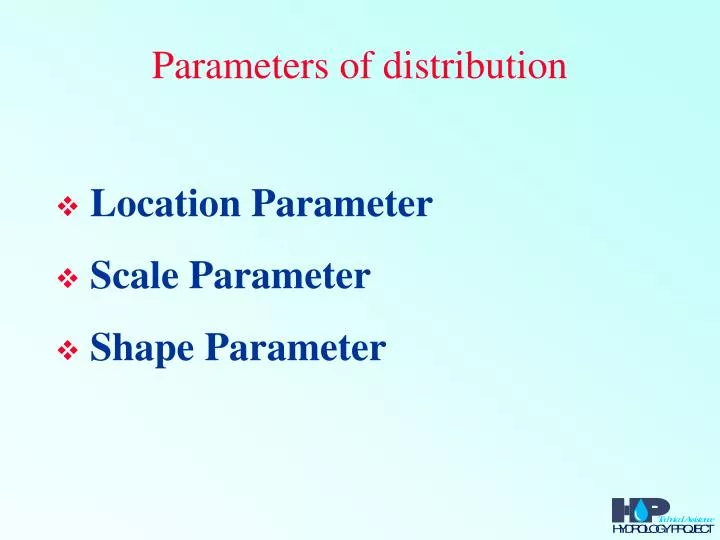
Parameters of distribution. Location Parameter Scale Parameter Shape Parameter. Plotting position. Plotting position of xi means, the probability assigned to each data point to be plotted on probability paper.

E N D
Parameters of distribution • Location Parameter • Scale Parameter • Shape Parameter
Plotting position • Plotting position of xi means, the probability assigned to each data point to be plotted on probability paper. • The plotting of ordered data on extreme probability paper is done according to a general plotting position function: • P = (m-a) / (N+1-2a). • Constant 'a' is an input variable and is default set to 0.3. • Many different plotting functions are used, some of them can be reproduced by changing the constant 'a'. • Gringorton P = (m-0.44)/(N+0.12) a = 0.44 • Weibull P = m/(N+1) a = 0 • Chegadayev P = (m-0.3)/(N+0.4) a = 0.3 • Blom P = (m-0.375)/(N+0.25) a = 0.375
Curve Fitting Methods • The method is based on the assumption that the observed data follow the theoretical distribution to be fitted and will exhibit a straight line on probability paper. • Graphical Curve fitting Method • Mathematical Curve fitting Method.- • Method of Moments- • Method of Least squares • Method of Maximum Likelihood
Estimation of statistical parameters (2) • Estimation procedures differ • Comparison of quality by: • mean square error or its root • error variance and standard error • bias • efficiency • consistency • Mean square error in of :
Estimation of statistical parameters (3) • Consequently: • First part is the variance of = average of squared differences about expected mean, it gives the random portion of the error • Second part is square of bias,bias= systematic difference between expected and true mean, it gives the systematic portion of the error • Root mean square error: • Standard error • Consistency: Mind effective number of data
Graphical estimation • Variable is function of reduced variate: • e.g. for Gumbel: • Reduced variate function of non-exceedance prob.: • Determine non-exceedance prob. from rank number of data in ordered set, e.g. for Gumbel: • Unbiased plotting position depends on distribution
Graphical estimation (2) • Procedure: • rank observations in ascending order • compute non-exceedance frequency Fi • transform Fi into reduced variate zi • plot xi versus zi • draw straight line through points by eye-fitting • estimate slope of line and intercept at z = 0 to find the parameters
Graphical estimation: example • Annual maximum river flow at Chooz on Meuse
Graphical estimation: example (2) • Gumbel parameters: • graphical estimation: x0 = 590, = 247 • MLM-method: x0 = 591, = 238 • 100-year flood: • T = 100 FX(x) = 1-1/100 = 0.99 • z = -ln(-ln(0.99)) = 4.6 • graphical method: x = x0 + z = 590 + 247x4.6 = 1726 m3/s • MLM method: x = x0 + z = 591 + 238x4.6 = 1686 m3/s • Graphical method: pro’s and con’s • easily made • visual inspection of series • strong subjective element in method: not preferred for design; only useful for first rough estimate • confidence limits will be lacking
Plotting positions • Plotting positions should be: • unbiased • minimum variance • General:
Censoring of data • Right censoring: eliminating data from analysis at the high side of the data set • Left censoring: eliminating data from analysis at the low side of the data set • Relative frequencies of remaining data is left unchanged. • Right censoring may be required because: • extremes in data set have higher T than follows from series • extremes may not be very accurate • Left censoring may be required because: • physics of lower part is not representative for higher values
Quantile uncertainty and conf. limits (2) • Confidence limits become: • CL diverge away from the mean • Number of data N also determine width of CL • Uncertainty in non-exceedance probability for a fixed xp: • standard error of reduced variate • It follows with zp approx N(zp,zp): hence:
Example rainfall Vagharoli (2) Normal distribution FX(z) for z=(x-877)/357 Ranked observations T=1/(1-FX(z)) Fi=(i-3/8)/(N+1/4)
Example Vagharoli (4) T FX(x) = 1 - 1/T
Investigating homogeneity • Prior to fitting, tests required on: • 1. stationarity (properties do not vary with time) • 2. homogeneity (all element are from the same population) • 3. randomness (all series elements are independent) • First two conditions transparent and obvious. Violating last condition means that effective number of data reduces when data are correlated • lack of randomness may have several causes; in case of a trend there will be serial correlation • HYMOS includes numerous statistical test : • parametric (sample taken from appr. Normal distribution) • non-parametric or distribution free tests (no conditions on distribution, which may negatively affect power of test
Summary of tests • On randomness: • median run test • turning point test • difference sign test • On correlation: • Spearman rank correlation test • Spearman rank trend test • Arithmetic serial correlation coefficient • Linear trend test • On homogeneity: • Wilcoxon-Mann-Whitney U-test • Student t-test • Wilcoxon W-test • Rescaled adjusted range test
Chi-square goodness of fit test • Hypothesis • F(x) is the distribution function of a population from which sample xi, i =1,…,N is taken • Actual to theoretical number of occurrences within given classes is compared • Procedure: • data set is divided in k class intervals containing at least each 5 values • Class limits from all classes have equal probability pj = 1/k = F(zj) - F(zj-1) e.g. for 5 classes this is p = 0.20, 0.40, 0.60, 0.80 and 1.00 • the interval j contains all xi with: UC(j-1)<xi UC(j) • the number of samples falling in class j = bj is computed • the number of values expected in class j = ej according to the theoretical distribution is computed • the theoretical number of values in any class = N/k because of the equal probability in each class
Chi-square goodness of fit test (2) • Consider following test statistic: • under H0 test statistic has 2 distr, with df = k-1-m • k= number classes, m = number of parameters • simplified test statistic: • H0 not rejected at significance level if:
Example • Annual rainfall Vagharoli (see parameter estimation) • test on applicability of normal distribution • 4 class intervals were assumed (20 data) • upper class levels are at p=0.25, 0.50, 0.75 and 1.00 • the reduced variates are at -0.674, 0.00, 0.674 and • hence with mean = 877, and stdv = 357 the class limits become: 877 - 0.674x357 = 636 877 = 877 877 + 0.674x357 = 1118
Example continued (2) From the table it follows for the test statistic: At significance level = 5%, according to Chi-squared distribution for = 4-1-2 df the critical value is at 3.84, hence c2 < critical value, so H0 is not rejected