Download
1 / 44
550 likes | 812 Vues
Statistical Parametric Mapping (SPM) 1. Talk I: Spatial Pre-processing 2. Talk II: General Linear Model 3. Talk III: Statistical Inference 3. Talk IV: Experimental Design. Spatial Preprocessing & Computational Neuroanatomy With thanks to:

E N D
Statistical Parametric Mapping (SPM) 1. Talk I: Spatial Pre-processing 2. Talk II: General Linear Model 3. Talk III: Statistical Inference 3. Talk IV: Experimental Design
Spatial Preprocessing & Computational Neuroanatomy With thanks to: John Ashburner, Jesper Andersson
Statistical Parametric Map Design matrix fMRI time-series kernel Motion correction Smoothing General Linear Model Spatial normalisation Parameter Estimates Standard template Overview
Overview 1. Realignment (motion correction) 2. Normalisation (to stereotactic space) 3. Smoothing 4. Between-modality Coregistration 5. Segmentation (to gray/white/CSF) 6. Morphometry (VBM/DBM/TBM)
Overview 1. Realignment (motion correction) 2. Normalisation (to stereotactic space) 3. Smoothing 4. Between-modality Coregistration 5. Segmentation (to gray/white/CSF) 6. Morphometry (VBM/DBM/TBM)
Reasons for Motion Correction • Subjects will always move in the scanner • The sensitivity of the analysis depends on the residual noise in the image series, so movement that is unrelated to the subject’s task will add to this noise and hence realignment will increase the sensitivity • However, subject movement may also correlate with the task… • …in which case realignment may reduce sensitivity (and it may not be possible to discount artefacts that owe to motion) • Realignment (of same-modality images from same subject) involves two stages: • 1. Registration - determining the 6 parameters that describe the rigid body transformation between each image and a reference image • 2. Transformation (reslicing) - re-sampling each image according to the determined transformation parameters
Squared Error Rigid body transformations parameterised by: Translations Pitch Roll Yaw 1. Registration • Determine the rigid body transformation that minimises the sum of squared difference between images • Rigid body transformation is defined by: • 3 translations - in X, Y & Z directions • 3 rotations - about X, Y & Z axes • Operations can be represented as affinetransformation matrices: x1 = m1,1x0 + m1,2y0 + m1,3z0 + m1,4 y1 = m2,1x0 + m2,2y0 + m2,3z0 + m2,4 z1 = m3,1x0 + m3,2y0 + m3,3z0 + m3,4
1. Registration • Iterative procedure (Gauss-Newton ascent) • Additional scaling parameter • Nx6 matrix of realignment parameters written to file (N is number of scans) • Orientation matrices in *.mat file updated for each volume (do not have to be resliced) • Slice-timing correction can be performed before or after realignment (depending on acquisition)
Nearest Neighbour Linear Full sinc (no alias) Windowed sinc 2. Transformation (reslicing) • Application of registration parameters involves re-sampling the image to create new voxels by interpolation from existing voxels • Interpolation can be nearest neighbour (0-order), tri-linear (1st-order), (windowed) fourier/sinc, or in SPM2, nth-order “b-splines”
Residual Errors after Realignment • Interpolation errors, especially with tri-linear interpolation and small-window sinc • PET: • Incorrect attenuation correction because scans are no longer aligned with transmission scan (a transmission scan is often acquired to give a map of local positron attenuation) • fMRI (EPI): • Ghosts (and other artefacts) in the image (which do not move as a rigid body) • Rapid movements within a scan (which cause non-rigid image deformation) • Spin excitation history effects (residual magnetisation effects of previous scans) • Interaction between movement and local field inhomogeniety, giving non-rigid distortion
New in SPM2 Field-map Distorted image Corrected image Unwarp • Echo-planar images (EPI) contain distortions owing to field inhomogenieties (susceptibility artifacts, particularly in phase-encoding direction) • They can be “undistorted” by use of a field-map (available in the “FieldMap” SPM toolbox) • (Note that susceptibility artifacts that cause drop-out are more difficult to correct) • However, movement interacts with the field inhomogeniety (presence of object affects B0), ie distortions change with position of object in field • This movement-by-distortion can be accommodated during realignment using “unwarp”
New in SPM2 Estimated derivative fields Pitch + B0 Roll Unwarp • One could include the movement parameters as confounds in the statistical model of activations • However, this may remove activations of interest if they are correlated with the movement • Better is to incorporate physics knowledge, eg to model how field changes as function of pitch and roll(assuming phase-encoding is in y-direction)… • … using Taylor expansion (about mean realigned image): • Iterate: 1) estimate movement parameters (, ), 2) estimate deformation fields, 1) re-estimate movement … • Fields expressed by spatial basis functions (3D discrete cosine set)…
New in SPM2 (0th-order term can be determined from fieldmap) + error + = + B0{i} fi f1 B0 - +2 1 i i + ... +5 + ... i Unwarp
New in SPM2 No correction Correction by covariation Correction by Unwarp tmax=13.38 tmax=5.06 tmax=9.57 Unwarp Example: Movement correlated with design
Overview 1. Realignment (motion correction) 2. Normalisation (to stereotactic space) 3. Smoothing 4. Between-modality Coregistration 5. Segmentation (to gray/white/CSF) 6. Morphometry (VBM/DBM/TBM)
Reasons for Normalisation • Inter-subject averaging • extrapolate findings to the population as a whole • increase statistical power above that obtained from single subject • Reporting of activations as co-ordinates within a standard stereotactic space • e.g. the space described by Talairach & Tournoux • Label-based approaches: Warp the images such that defined landmarks (points/lines/surfaces) are aligned • but few readily identifiable landmarks (and manually defined?) • Intensity-based approaches: Warp to images to maximise some voxel-wise similarity measure • eg, squared error, assuming intensity correspondence (within-modality) • Normalisation constrained to correct for only gross differences; residual variabilility accommodated by subsequent spatial smoothing
Summary Spatially normalised Original image • Determine transformation that minimises the sum of squared difference between an image and a (combination of) template image(s) • Two stages: • 1. affine registration to match size and position of the images • 2. non-linear warping to match the overall brain shape • Uses a Bayesian framework to constrain affine and warps Spatial Normalisation Template image Deformation field
Rigid body Rotation Shear Translation Zoom Stage 1. Full Affine Transformation • The first part of normalisation is a 12 parameter affine transformation • 3 translations • 3 rotations • 3 zooms • 3 shears • Better if template image in same modality (eg because of image distortions in EPI but not T1)
Six affine registered images Insufficieny of Affine-only normalisation Six affine + nonlinear registered
Stage 2. Nonlinear Warps • Deformations consist of a linear combination of smooth basis images • These are the lowest frequency basis images of a 3-D discrete cosine transform • Brain masks can be applied (eg for lesions)
Template image Affine Registration (2 = 472.1) Non-linear registration with regularisation (2 = 302.7) Non-linear registration without regularisation (2 = 287.3) Bayesian Constraints Without the Bayesian formulation, the non-linear spatial normalisation can introduce unnecessary warping into the spatially normalised images
Bayesian Constraints • Using Bayes rule, we can constrain (“regularise”) the nonlinear fit by incorporating prior knowledge of the likely extent of deformations: • p(p|e) p(e|p) p(p) (Bayes Rule) • p(p|e) is the a posteriori probability of parameters p given errors e • p(e|p) is the likelihood of observing errors e given parameters p • p(p) is the a priori probability of parameters p • For Maximum a posteriori (MAP) estimate, we minimise (taking logs): • H(p|e) H(e|p) + H(p) (Gibbs potential) • H(e|p) (-log p(e|p)) is the squared difference between the images (error) • H(p)(-log p(p)) constrains parameters (penalises unlikely deformations) • is “regularisation” hyperparameter, weighting effect of “priors”
Empirically generated priors Bayesian Constraints • Algorithm simultaneously minimises: • Sum of squared difference between template and object • Squared distance between the parameters and their expectation • Bayesian constraints applied to both: 1) affine transformations • based on empirical prior ranges 2) nonlinear deformations • based on smoothness constraint (minimising membrane energy)
Overview 1. Realignment (motion correction) 2. Normalisation (to stereotactic space) 3. Smoothing 4. Between-modality Coregistration 5. Segmentation (to gray/white/CSF) 6. Morphometry (VBM/DBM/TBM)
FWHM Gaussian smoothing kernel Reasons for Smoothing • Potentially increase signal to noise (matched filter theorem) • Inter-subject averaging (allowing for residual differences after normalisation) • Increase validity of statistics (more likely that errors distributed normally) • Kernel defined in terms of FWHM (full width at half maximum) of filter - usually ~16-20mm (PET) or ~6-8mm (fMRI) of a Gaussian • Ultimate smoothness is function of applied smoothing and intrinsic image smoothness (sometimes expressed as “resels” - RESolvable Elements)
Overview 1. Realignment (motion correction) 2. Normalisation (to stereotactic space) 3. Smoothing 4. Between-modality Coregistration 5. Segmentation (to gray/white/CSF) 6. Morphometry (VBM/DBM/TBM)
T1 Transm T2 PD PET EPI Between Modality Co-registration • Because different modality images have different properties (e.g., relative intensity of gray/white matter), cannot simply minimise difference between images • Two main approaches: I. Via Templates: 1) Simultaneous affine registrations between each image and same-modality template 2) Segmentation into grey and white matter 3) Final simultaneous registration of segments II. Mutual Information • Useful, for example, to display functional results (EPI) onto high resolution anatomical image (T1)
Between Modality Co-registration: I. Via Templates 3. Registration of Partitions 1. Affine Registrations • ‘Mixture Model’ cluster analysis to classify MR image as GM, WM & CSF • Additional information is obtained from a priori probability images - see later • Both images are registered - using 12 parameter affine transformations - to their corresponding templates... • … but only the rigid-body transformation parameters allowed to differ between the two registrations • This gives: • rigid body mapping between the images • affine mappings between the images and the templates 2. Segmentation • Grey and white matter partitions are registered using a rigid body transformation • Simultaneously minimise sum of squared difference
New in SPM2 Another way is to maximise the Mutual Information in the 2D histogram (plot of one image against other) For histograms normalised to integrate to unity, the Mutual Information is: SiSj hij log hij Sk hikSl hlj PET T1 MRI Between Modality Coregistration: II. Mutual Information
Overview 1. Realignment (motion correction) 2. Normalisation (to stereotactic space) 3. Smoothing 4. Between-modality Coregistration 5. Segmentation (to gray/white/CSF) 6. Morphometry (VBM/DBM/TBM)
Priors: Intensity histogram fit by multi-Gaussians . Image: GM WM CSF Brain/skull Image Segmentation • Partition into gray matter (GM), white matter (WM) and cerebrospinal fluid (CSF) • ‘Mixture Model’ cluster analysis used, which assumes each voxel is one of a number of distinct tissue types (clusters), each with a (multivariate) normal distribution • Further Bayesian constraints fromprior probability images, which are overlaid • Additional correction for intensity inhomogeniety possible
Overview 1. Realignment (motion correction) 2. Normalisation (to stereotactic space) 3. Smoothing 4. Between-modality Coregistration 5. Segmentation (to gray/white/CSF) 6. Morphometry (VBM/DBM/TBM)
Original Template Spatial Normalisation Normalised Deformation field TBM VBM DBM Morphometry (Computational Neuroanatomy) • Voxel-by-voxel: where are the differences between populations? • Univariate: e.g, Voxel-Based Morphometry (VBM) • Multivariate: e.g, Tensor-Based Morphometry (TBM) • Volume-based: is there a difference between populations? • Multivariate: e.g, Deformation-Based Morphometry (DBM) • Continuum: • perfect normalisation => all information in Deformation field (no VBM differences) • no normalisation => all in VBM
Spatially normalised Segmented grey matter Original image Smoothed SPM Voxel-Based Morphometry (VBM) A voxel by voxel statistical analysis is used to detect regional differences in the amount of grey matter between populations “Optimised” VBM involves segmenting images before normalising, so as to normalise gray matter / white matter / CSF separately...
T1 image template Optimised VBM Affine registration Affine transform priors Segmentation & Extraction STATS volume smooth Spatial normalisation Modulation Apply deformation Segmentation & extraction Normalised T1 STATS concentration smooth
Grey matter volume loss with age superior parietal pre and post central insula cingulate/parafalcine VBM Examples: Aging
Females > Males Males > Females L superior temporal sulcus R middle temporal gyrus intraparietal sulci mesial temporal temporal pole anterior cerebellar VBM Examples: Sex Differences
Right frontal and left occipital petalia VBM Examples: Brain Asymmetries
Vector field Tensor field Morphometry on deformation fields: DBM/TBM Deformation-based Morphometry looks at absolute displacements Tensor-based Morphometry looks at local shapes
Deformation fields ... Remove positional and size information - leave shape Parameter reduction using principal component analysis (SVD) Multivariate analysis of covariance used to identify differences between groups Canonical correlation analysis used to characterise differences between groups Deformation-based Morphometry (DBM)
Non-linear warps of sex differences characterised by canonical variates analysis Mean differences (mapping from an average female to male brain) DBM Example: Sex Differences
Original Warped Template Relative volumes Strain tensor Tensor-based morphometry If the original Jacobian matrix is donated by A, then this can be decomposed into: A = RU, where R is an orthonormal rotation matrix, and U is a symmetric matrix containing only zooms and shears. Strain tensors are defined that model the amount of distortion. If there is no strain, then tensors are all zero. Generically, the family of Lagrangean strain tensors are given by: (Um-I)/m when m~=0, and log(U) if m==0.
References Friston et al (1995): Spatial registration and normalisation of images.Human Brain Mapping 3(3):165-189 Ashburner & Friston (1997): Multimodal image coregistration and partitioning - a unified framework.NeuroImage 6(3):209-217 Collignon et al (1995): Automated multi-modality image registration based on information theory.IPMI’95 pp 263-274 Ashburner et al (1997): Incorporating prior knowledge into image registration.NeuroImage 6(4):344-352 Ashburner et al (1999): Nonlinear spatial normalisation using basis functions.Human Brain Mapping 7(4):254-266 Ashburner & Friston (2000): Voxel-based morphometry - the methods.NeuroImage 11:805-821