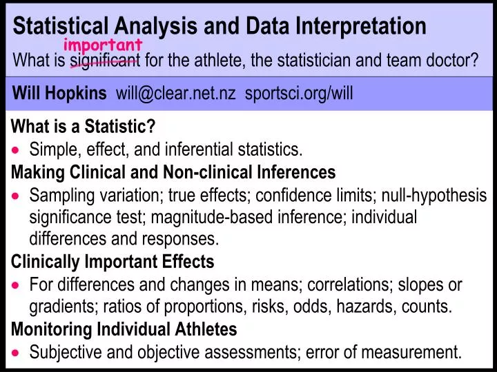
Will Hopkins will@clear.net.nz sportsci.org/will

1. Will Hopkins will@clear.net.nz sportsci.org/will Statistical Analysis and Data InterpretationWhat is significant for the athlete, the statistician and team doctor? important What is a Statistic? • Simple, effect, and inferential statistics. Making Clinical and Non-clinical Inferences • Sampling variation; true effects; confidence limits; null-hypothesis significance test; magnitude-based inference; individual differences and responses. Clinically Important Effects • For differences and changes in means; correlations; slopes or gradients; ratios of proportions, risks, odds, hazards, counts. Monitoring Individual Athletes • Subjective and objective assessments; error of measurement.

2. What is a Statistic? • Definition: a number summarizingan aspect of many numbers. • Examples: mean, correlation, confidence limit… • If the many numbers all represent different values of the same kind of thing, we call the numbers values of a numericvariable. • Example: 57, 73, 61, 60 kg are values of the variable body mass. • Values of a variable all have the same units. • A nominal or groupingvariable has levelsor labels rather than numeric values. • Example: union, league, touch… are levels of the variable rugby. • Utility: a statistic usually represents the bigpicture or some other important aspect of the original numbers. • The aspect is often not obvious in the original numbers. • One number is better than many. • Most people hate numbers. The fewer, the better!

3. Simple statistic: an aspect of a set of values of one variable. • Sample size (n): the number of values. • Mean: the average value or center of the values. • Standarddeviation (SD): the average scatter around the mean. • Used to evaluate magnitudes of differences in means. • Standard error of the mean (SD/n): the expected variation in the mean with resampling. • A tricky statistical dinosaur. Avoid! • Convert back to the SD when you see it. • Quantiles (median, tertiles, quartiles, quintiles…): values that divide the ranked set up into 2, 3, 4, 5… equal-sized subsets. • Used when the set is skewed by large values (e.g., salaries). • Also used to compare subgroups. Example: systolic pressure in the quintile of lowest physical activity vs each quintile of higher activity. • Proportion or risk: the number of "events" (e.g., injured players) divided by the number of "trials" (total number of players). • Often expressed as a percent (proportion×100).

4. Effect statistic: a relationship between a predictor or independent variable and a dependent or outcome variable. • Difference (or change) in mean: the predictor is a grouping variable and the dependent is numeric. • Slope (or gradient): the difference or change in the mean per difference in a numeric predictor. • Correlationcoefficient: another form of the slope. • Ratio of proportions, risks, odds or hazards: statistics for comparing the occurrence (presence or absence) of something in two groups. • Ratio of counts: statistics for comparing counts or occurrences of something in two groups. • Other variables can be included in the analysis as covariates. • Moderators are interacted with the predictor to estimate how the effect differs between subjects. • Mediators are added to adjust for effects of subject characteristics, which means: "for subjects of the same age…, the effect was…". Such adjustment also deals with potential confounding(by age…).

5. Inferentialstatistic: an aspect of the "true" value of a simple or effect statistic derived from a sample. • Confidenceinterval or limits: the likely range of the true value. • P value: provides evidence about the zero or null value of an effect. • Chance of benefit, risk of harm: provide evidence about the true value for making clinical decisions. • T, F, chi-squared statistics: "test" statistics used to get the above. • Only the statistician needs to know about these. • They shouldn’t be shown in publications.

6. Making Clinical Inferences (Decisions or Conclusions)c • Every sample gives a different value for a statistic, owing to sampling variation. • So, the value of a sample statistic is only an estimate of the true (right, real, actual, very large sample, or population) value. • But people want to make an inference about the true value. • The best inferential statistic for this purpose is the confidenceinterval: the range within which the true value is likely to fall. • "Likely" is usually 95%, so there is a 95% chance the true value is included in the confidence interval (and a 5% chance it is not). • Confidence limits are the lower and upper ends of the interval. • The limits represent how small and how large the effect "could" be. • All effects should be shown with a confidence interval or limits. • Example: the dietary treatment produced an average weight loss of 3.2 kg (95% confidence interval 1.6 to 4.8 kg). • The confidence interval is NOT a range of individual responses! • But confidence limits alone don't provide a clinical inference.

7. zero or null • Statistical significanceis the traditional way to make inferences. • Also known as the null-hypothesis significance test. • The inference is all about whether the effect could be zero or "null". • If the 95% confidence interval includes zero, the effect "could be zero". The effect is "statistically non-significant (at the 5% level)": • If the confidence interval does not include zero, the effect "couldn't be zero". The effect is "statistically significant (at the 5% level)". • Stats packages calculate a probability or p value for deciding whether an effect is significant. • p>0.05 means non-significant; p<0.05 means significant. negative positive Researchers using p values should show exact values. 95% confidence interval (p=0.31) statistically non-significant statistically significant (p=0.02) (p=0.003) statistically significant value of effect statistic (e.g., change in weight)

8. The exact definition of the p value is hard to understand. • Useful interpretation: half the p value is the probability the true effect is negative when the sample effect is positive (and vice versa). • People usually interpret non-significant as "no real effect" and significant as "a real effect". • These interpretations apply only if the study was done with the right sample size. • Even then they are misleading: they don't convey the uncertainty. • And you hardly ever know if the sample size is right. • Attempts to address this problem with post-hoc power calculations are rare, generally wrong, and too hard to understand. • So the only safe interpretation is whether the effect could be zero. • But the issue for the practitioner is not whether the effect could be zero, but whether the effect could be important. • Important has two meanings: beneficial and harmful. • The confidence interval addresses this issue, when clinically important values for benefit and harm are taken into account.

9. Clinicaldecision Clear: don't use it. smallest clinicallybeneficial effect smallest clinicallyharmful effect Clear: don't use it. • Clinical inferences with the confidence interval • The smallest clinically important effects define values of the effect that are beneficial, harmful and trivial. • Smallest effects for benefit and harm are equal and opposite. • Infer (decide) the outcome from the confidence interval, as follows: P values fail here. harmful trivial beneficial Clear: use it. Clear: use it. Clear: use it. But p>0.05! Clear: depends. Clear: don't use it. But p<0.05! Unclear: more data needed. value of effect statistic (e.g., change in weight)

10. This approach obviates any need for statistical significance. • The only issue is what level to make the confidence interval. • To be careful about avoiding harm, you can make a conservative 99% confidence interval on the harm side. • And to use effects only when there is a reasonable chance of benefit. you can make a 50% interval on the benefit side. • But that's hard to understand. Consider this equivalent approach… • Clinical inferences with probabilities of benefit and harm. • The uncertainty in an effect can be expressed as chances that the true effect is beneficial and the risk that it is actually harmful. • You would decide to use an effect with a reasonable chance of benefit, provided it had a sufficiently low risk of harm. • I have opted for possibly beneficial (>25% chance of benefit) and most unlikely harmful (<0.5% chance of harm). • An effect with >25% chance of benefit and >0.5% risk of harm is therefore unclear. You'd like to use it, but you daren't. • Everything else is either clearly useful or clearly not worth using.

11. If the chance of benefit is high (e.g., 80%), you could accept a higher risk of harm (e.g., 5%). • This less conservative approach has been formalized using a threshold odds ratio of 66 (odds of benefit to odds of harm). • When an effect has no obvious benefit or harm (e.g., a comparison of males and females), the inference is only about whether the effect could be substantially positive or negative. • For such non-clinical inferences, use a symmetrical confidence interval, usually 90% or 99%, to decide whether the effect is clear. • Equivalently, one or other of the chances of being substantially positive or negative has to be <5% for the effect to be clear ("a clear non-clinical effect can't be substantially positive and negative"). • Ways to report inferences for clear effects: possibly small benefit, likely moderately harmful, a large difference (clear at 99% level), a trivial-moderate increase [the lower and upper confidence limits]… • Whatever, researchers should make a magnitude-based inference by showing confidence limits and interpreting the uncertainty in a (clinically) relevant way readers can understand.

12. A caution about making an inference… • Whatever method you use, the inference is about theone and only mean effect in the population. • The confidence interval represents the uncertainty in the true effect, not a range of individual differences or individual responses. • For example, with a large-enough sample size, a treatment could be clearly beneficial (a mean beneficial effect with a narrow confidence interval), yet the treatment could be harmful for a substantial proportion of the population. • Individual differences between groups and individual responses to a treatment are best summarized with a standard deviation to go with the mean effect. • The mean effect and the SD both need confidence limits. • Individual differences between groups and individual responses to a treatment may be accounted for by including subject characteristics as modifying covariates in the analysis. • Researchers generally neglect this important issue.

13. Clinically Important Magnitudes of Effects • Researchers and practitioners need to know about clinically important magnitudes to interpret research findings. • Researchers need the smallest clinically important magnitude of an effect statistic to estimate sample size for a study. • For those who use the null-hypothesis significance test, the right sample size has 80% power (80% chance of statistical significance, p<0.05) if the true effect has the smallest important value. • For those who use clinical magnitude-based inference, the right sample size gives a 0.5% risk of harm and a 25% chance of benefit if the true effect has the smallest important beneficial value. • Practitioners need to know about clinically important magnitudes to monitor their athletes or patients. • So the next few slides are all about values for various magnitudes of various effect statistics.

14. Strength patients healthy Data are means & SD. Strength pre post1 post2 Trial Differences or Changes in the Mean • The most common effect statistic, for numberswith decimals (continuous variables). • Difference when comparing different groups, e.g., patients vs healthy. • In population-health studies, groups are oftensubdivided into quartiles or quintiles (e.g., of age). • Change when tracking the same subjects. • Difference in the changes in controlled trials. • The between-subject standard deviationprovides default thresholds for importantdifferences and changes. • You think about the effect (mean) in terms of afraction or multiple of the SD (mean/SD). • The effect is said to be standardized. • The smallest important effect is ±0.20 (±0.20 of an SD). Data are means & SD.

15. Trivial effect (0.1x SD) Very large effect (3.0x SD) post post pre pre Cohen Hopkins trivial <0.2 <0.2 small moderate 0.5-0.8 0.6-1.2 Complete scale: large >0.8 1.2-2.0 extremely large strength strength 0.2 0.6 1.2 2.0 4.0 trivial small moderate large very large ext. large very large ? ? 2.0-4.0 >4.0 • Example: the effect of a treatment on strength • Interpretation of standardizeddifference orchange in means: 0.2-0.5 0.2-0.6

16. Cautions with standardizing • Standardizing works only when the SD comes from a sample that is representative of a well-defined population. • The resulting magnitude applies only to that population. • In a controlled trial, use the baseline (pre) SD, never the SD of change scores. • Beware of authors who show standard errors of the mean (SEM) rather than standard deviations (SD). • SEM = SD/(sample size), so SEMs on graphs make effects look a lot bigger than they really are. • Very rarely, overlap of SEM of two groups indicates that the difference between the means is not statistically significant. • But you won't know when that applies, and you're not using or trusting statistical significance anymore anyway, right? • Standardization may not be best for effects on means of some special variables: visual-analog scales, Likert scales, solo athletic performance…

17. Visual-analog scales • The respondents indicate a perception on a line like this: Rate your pain by placing a mark on this scale: • Score the response as percent of the length of the line. • Magnitude thresholds: 10%, 30%, 50%, 70%, 90% for small, moderate, large, very large, extremely large differences or changes. • Likert scales • These are used for responses to questions like this: Over the last four weeks, how often did you train in a gym? not at allonce only2-3 timesonce a weektwice or more a week • Most Likert-type questions have four to seven choices. • Code them as integers (1, 2, 3, 4, 5…) and analyze as numerics. • Magnitude thresholds are up for debate. • If you use the thresholds of the visual-analog scale as a guide, the threshold for a 6-pt scale would be ~0.5, 1.5, 2.5, 3.5 and 4.5.   none unbearable

18. Solo athleticperformance • For fitness tests of team-sport athletes, use standardization. • But for top solo athletes, an enhancement that results in one extra medal per 10 competitions is the smallest important effect. • The within-athlete variability that athletes show from one competition to the next determines this effect. Here's why… • Owing to this variability, each of the top athletes has a good chance of winning at each competition: Race 1 Race 2 Race 3

19. 0.3 0.9 1.6 2.5 4.0 trivial small moderate large very large ext. large • Your athlete needs an enhancement that overcomes this variability to give her or him a bigger chance of a medal. • Simulations show an enhancementof 0.3 of an athlete's typical variability from competition to competition givesone extra win every 10 competitions. • Example: if the variability is an SD (coefficient of variation) of 1%, the smallest important enhancement is 0.3%. • In some early publications I have mistakenly referred to 0.5 of the variability as the smallest effect. • Small, moderate, large, very large and extremely large effects result in an extra 1, 3, 5, 7 and 9 medals in every 10 competitions. • The corresponding enhancements as factors of the variabilityare:

20. Beware: smallest effect on athletic performance in performance tests depends on method of measurement, because… • A percent change in an athlete's ability to output power results in different percent changes in performance in different tests. • These differences are due to the power-duration relationship for performance and the power-speed relationship for different modes of exercise. • Example: a 1% change in endurance power output produces the following changes… • 1% in running time-trial speed or time; • ~0.4% in road-cycling time-trial time; • 0.3% in rowing-ergometer time-trial time; • ~15% in time to exhaustion in a constant-power test. • A hard-to-interpret change in any test following a fatiguing pre-load. (But such tests can be interpreted for cycling road races: see Bonetti and Hopkins, Sportscience 14, 63-70, 2010.)

21. Physical activity Age Slope (or Gradient) • Used when the predictor and dependent are both numeric and a straight line fits the trend. • The unit of the predictor is arbitrary. • Example: a 2% per year decline in activity seems trivial… yet 20% per decade seems large. • So it's best to express a slope as thedifference in the dependent per two SDs of predictor. • It gives the difference in the dependent (physical activity) between a typically low and high subject. • The SD for standardizing the resulting effect is the standard error of the estimate (the scatter about the line). 2 SD

22. Correlation Coefficient • Closely related to the slope, this represents the overall linearity in a scatterplot. Examples: • Negative values represent negative slopes. • The value is unaffected by the scaling of the two variables or by the sample size. • And it's much easier to calculate than a slope. • But a properly calculated slope is easier to interpret clinically. • Smallest important correlation is ±0.1. Complete scale: r = 0.00 r = 0.10 r = 0.30 r = 0.50 r = 0.70 r = 0.90 r = 1.00 0.1 0.3 0.5 0.7 0.9 trivial low moderate high very high ext. high

23. Differences and Ratios of Proportions, Risks, Odds, Hazards • Example: percent of male and female players injured at allin a season of touch rugby. • Risk difference or proportion difference • A common measure. Example: a-b = 75%-36% = 39%. • Problem: the sense of magnitude of a given difference depends on how big the proportions are. • Example: for the same 10% difference,90% vs 80% doesn't seem big, but… 11% vs 1% can be interpreted as a huge "difference" (11x the risk). • So there is no scale of magnitudes for a risk or proportion difference. • And analyses (models) don't work properly with proportions. • We have to use odds or hazards instead of proportions. Stay tuned. Proportioninjured (%) 100 a =75% b =36% 0 male female Sex

24. Proportioninjured (%) 100 a =75% • Number needed to treat (NNT) = 100/(risk difference (%)). • The number you would have to treat or sample for one subject to have an outcome attributable to the effect. • Has been promoted in some clinical journals, but not widely used. • Hard to analyze properly. • Problems with its confidence limits. • Avoid! • Risk ratio (relative risk) or proportion ratio • Another common measure.Example: a/b = 75/36 = 2.1, which meansmales are "2.1 times more likely" to be injured,or "a 110% increase in risk" of injury for males. • Problem: if it's a time dependent measure, the riskratio changes. • If you wait long enough, everyone gets affected, so risk ratio = 1.00. • But it works for rare time-dependent risks and for time-independent classifications (e.g., proportion playing a sport). b =36% 0 male female Sex

25. 1.11 1.43 2.0 3.3 10 trivial small moderate large very large ext. large • Smallest important effect for risk or proportion ratio:for every 10 injured males there are 9 injured females. • That is, one in 10 injuries is due to being male. • If there are N males and N females, risk ratio = (10/N)/(9/N) = 10/9. • Similarly, moderate, large, very large and extremely large effects:for every 10 injured males, there are 7, 5, 3 and 1 injured females. • Corresponding risk ratios are 10/7, 10/5, 10/3 and 10/1. • Hence complete scale for proportion ratio and low-risk ratio: • and the inverses for reductions in proportions: 0.9, 0.7, 0.5, 0.3, 0.1. • But there is still the problem of analyzing proportions properly. • Two solutions: hazards instead of risks; odds instead of proportions.

26. Hazard ratio for time-dependent events. • To understand hazards, consider theincrease in proportion or risk with time. • The hazard is the tiny proportionthat gets affected per a tiny interval of time. • Example: hazard for males = a = 0.28% per day,hazard for females = b = 0.11% per day. So hazard ratio = a/b = 0.28/0.11 = 2.5. • That is, males are 2.5x more likely to get injuredper unit time, whatever the (small) unit of time. • So you could call it the "right-now risk ratio". • It's also known as incidence rate ratio, which is the ratio of the slopes. • It can also be interpreted as the ratio of the times taken for the same proportion to get affected in two groups. • Example: females take 2.5x as long to get injured as males. Proportioninjured (%) 100 males females 0 Time (months) a b 1day

27. a b 1.11 1.43 2.0 3.3 10 trivial small moderate large very large ext. large 100 males • Hazard ratios work over long periods, when a substantial proportion of males or females is injured, and the observed risk ratio drops below the initial hazard ratio. • Example: at 5 weeks, the risk ratio = a/b = 75/36 = 2.1. • But the hazard ratio for those still uninjured is usually assumed to stay the same, even if the hazards change with time. • Example: the risk of injury might increase laterin the season for both sexes, but the right-now risk ratio for new injuries (the hazard ratio) doesn't change. A big plus! • And hazards and hazard ratios can be modeled (analyzed)! • Magnitude thresholds must be the same as for the proportion ratio, even for frequent events, because such events start off rare. • Hence this scale for the hazard ratio: • and the inverses 0.9, 0.7, 0.5, 0.3, 0.1. Proportioninjured (%) females 0 Time (months)

28. Proportionplaying (%) 100 c =25% d =64% a =75% • Odds ratio for time-independent classifications. • Classifications refer to prevalence; risks refer to incidence. • Odds are the awkward but only way to model classifications. • Example: proportions of boys and girlsplaying a sport. • Odds of a boy playing = a/c = 75/25. • Odds of a girl playing = b/d = 36/64. • Odds ratio = (75/25)/(36/64) = 5.3. • Interpret the ratio as "…times more likely" only when the proportions in both groups are small (<10%). • The odds ratio is then approximately equal to the proportion ratio. • To assess magnitude, authors should convert the odds ratio and its confidence limits to the proportion ratio and its confidence limits. • Unfortunately they often just leave effects as odds ratios. b =36% 0 boys girls Sex

29. 1.11 1.43 2.0 3.3 10 trivial small moderate large very large ext. large Ratio of Counts • Example: 93 vs 69 injuries per 1000 player-hours of match play in sport A vs sport B. • The effect is expressed as a ratio: 93/69 = 1.35x more injuries. • Can also be expressed as 35% more injuries. • The scale of magnitudes is the same as for ratio of proportions: • and the inverses 0.9, 0.7, 0.5, 0.3, 0.1. –––––––––– • Effects of numeric linear predictors (slopes) for ratio outcomes are expressed as risk, odds, hazard or count ratios per unit of the predictor and evaluated as the effect per 2 SD of the predictor.

30. Modeling Effects • Estimates and inferential statistics for mean effects and slopes come from various kinds of general linear model… • t tests, simple and multiple linear regression, ANOVA… • Use mixed linear models for repeatedmeasures and clustering. • Testing for normality is pointless, but uniformity is the real issue. • Many effects are more uniform when estimated as percents or ratios via analysis of the log-transformed dependent variable. • Bootstrapping of confidence limits works with difficult data. • Ratios of odds, hazards and counts need various kinds of generalizedlinear model… • All include log transformation to estimate ratios. • Logistic (log-odds) regression for odds, log-hazard and Cox regression for hazards, Poisson regression for counts. • And don't forget that covariates in all these models estimate and adjust for effects of moderators and mediators or confounders.

31. Monitoring Individual Athletes • It’s all about a substantial change since the last assessment. • The subjective assessments (perceptions) of the athlete, coach, and support personnel provide important evidence. • One-off assessments often differ between individual practitioners, but assessments of change usually have high validity. • Objective assessments of change with an instrument or test are contaminated with error or "noise". • The noise is represented by the standard deviation of repeated measurements, the standard (or typical) error of measurement. • Think of ± the error as the equivalent of confidence limits for the athlete's true change. • Take into account clinically or practically important changes. • Wow, you've made a moderate improvement! • No real change either way. [A good instrument needed for this.] • Uh… unclear whether you’re getting better or worse.

32. Summary • Inferential statistics are used to make conclusions about the truevalue of a simple or effect statistic derived from a sample. • The inference from a null-hypothesis significance test is about whether the true value of an effect statistic could be null (zero). • Magnitude-based inference addresses the issue of whether the true value could be important (beneficial and harmful, or substantial). • Effect magnitudes have key roles in research and practice. • Effects for continuous dependents are mean differences, slopes (expressed per 2 SD of the predictor), and correlations. • Thresholds for small, moderate, large, very large and extremely large standardized mean differences: 0.20, 0.60, 1.2, 2.0, 4.0. • Thresholds for correlations: 0.10, 0.30, 0.50, 0.70, 0.90. • Magnitude thresholds for ratios of proportions, hazards, counts: 1.11, 1.43, 2.0, 3.3, 10 and their inverses 0.9, 0.7, 0.5, 0.3, 0.1. • Take noise and thresholds into account when monitoring athletes.