Chapter 5a: Functions of Random Variables

1. Chapter 5a: Functions of Random Variables zlyang@smu.edu.sg http://www.mysmu.edu/faculty/zlyang/ Yang Zhenlin

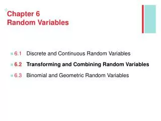
2. Chapter 5a Contents The main purpose of this chapter: Introducing methods for finding the distribution of a function of the random variable(s). Functions of One Random Variable --- change of variable technique Functions of Two Random Variables --- change of variable technique Sum of Independent Random variables --- The Moment Generating Function Technique

3. Functions of One Random Variable The case of a continuous random variable. Definition 5a.1 (Change-of-Variable Technique)Let X be a continuous type random variable with pdf f(x). Let Y = u(X) be a one-to-one transformation of X with inverse function X = v(Y). Then the pdf of Y is given by g(y) = f[v(y)] |v(y)|, where v(y) is the derivative of v(y). If the possible values of X are c1< x <c2, then the possible values of Y are u(c1)< y <u(c2). Example 5a.1. Let X have a gamma distribution with pdf Let Y = eX. Find the pdf of Y.

4. Functions of One Random Variable Solution: Since the inverse function is X= v(Y) = log (Y), v(y) = 1/y. Thus, by Definition 5.1, the pdf of Y is given by Since the support of X is (0, ), the support of Y is (1, ). The pdf of Y is thus, The way to see the change-of-variable technique is through CDF: G(y) = P{Y y} = P{X  v(y)} = F[v(y)]. Taking derivatives leads to g(y) = f[v(y)] |v(y)|. So, the change-of-variable technique is essentially the CDF technique.

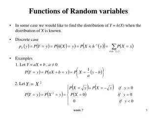
5. Functions of One Random Variable The case of a discrete random variable. • The Change-of-variable technique can be applied to a random variable X of the discrete type, but there is major difference: pmf p(x) = P{X = x} represents probability, but pdf f(x) does not. • For a one-to-one transformation, Y = u(X), with inverse X = v(Y), we can easily see that the pmf g(y) of Y is • g(y) = P{Y = y} = P{X = v(y)} = p[v(y)] • The possible values of Y are found directly from the possible values of X through the functional relation Y = u(X). Example 5a.2. Let X have a Poisson distribution with  = 4. Find the pmf of Y = X1/2. Since X = Y2, we have,

6. Functions of One Random Variable The case of a non-one-to-one function of a continuous r.v. • The change-of-variable technique requires that the function is one-to-one, thus cannot be applied when the function is not one-to-one. • However, as noted earlier, the distribution of functions of a random variable are essentially developed from the CDF. Thus, the distribution of a non-one-to-one function can still be derived from the CDF! • We will demonstrate this idea by showing an important result: The square of a standard normal random variable is a gamma r.v. with parameters (1/2, 2), this special gamma r.v. is called the chi-squared random variable with degrees of freedom equal to 1.

7. Functions of One Random Variable Example 5a.3. Let Z be a standard normal r.v. and let X = Z2. The CDF of X is Taking derivative with respect to x, we obtain the pdf of X: Recognizing that , the above is the pdf of a gamma r.v. with parameters (1/2, 2), called the chi-squared with 1 d.f.

8. Functions of Two Random Variables The above change-of-variable technique can be extended to the case of joint distributions involving two or more random variables. Many interesting problems solved. Definition 5a.2. (Change-of-Variable Technique)Let X1and X2be two continuous type random variables with joint pdf f(x1, x2). Let Y1 = u1(X1, X2) and Y2 = u2(X1, X2) be two continuous functions, which have single-valued inverse: X1 = v1(Y1, Y2) and X2 = v2(Y1, Y2). Then the joint pdf of Y1 and Y2 is where J, called the Jacobian, is the determinant of the matrix of partial derivatives:

9. Functions of Two Random Variables • Example 5a.4. Let X1 and X2 be two independent r.v.s, each with pdf f(x) = ex, 0 < x < . Consider Y1 = X1 X2,and Y2= X1 + X2. • Find the joint pdf of Y1and Y2 • Find the marginal pdfs of Y1and Y2, respectively.

10. Functions of Two Random Variables • where the possible values of Y1 and Y2 can be found as follows: • Y2= X1 + X2 implies 0 < Y2 < ; • X1=(Y1 + Y2)/2 > 0 implies Y1 > Y2; • X2=(Y2Y1)/2 > 0 implies Y1 < Y2. y2 The region of (Y1, Y2) values y2 = -y1 y2 = y1 y1

11. Functions of Two Random Variables • The marginal pdf of Y2: The marginal pdf of Y1: The latter expression can simply be written as That is called the double exponential pdf.

12. Functions of Two Random Variables Definition 5a.3. Let X and Y be jointly distributed r.v.s with joint pmf p(x, y), or a joint pdf f(x, y). Let u(X, Y) be a continuous function of X and Y. Then, u(X, Y) is also a random variable. If X and Y are both discrete, And if X and Y are both continuous, If X and Y are jointly distributed r.v.s, then, Var(X + Y) = Var(X) + Var(Y) + 2Cov(X, Y) If further X and Y are independent, then Var(X + Y) = Var(X) + Var(Y)

13. Functions of Two Random Variables Example 5a.5. The joint probability distribution of variables X and Y is shown in the table below, (a) Determine the marginal probability distributions of X and Y. (b) Are X and Y independent? Explain. (c) Find the probability mass function of X+Y. (d) Find the probability of P(XY). Solution: (a) The marginal pmfs are:

14. Functions of Two Random Variables • No. Because p(1, 1) = 0.20, but = 0.420.50 = 0.21. • Let Z = X+Y, then the pmf of Z is • Where, for example, • pZ(3) = P(X+Y = 3) = P(X = 1, Y = 2) + P(X = 2, Y = 1) • = 0.15 + 0.18 = 0.33. • (d) P(XY) = 1 P(X = Y) • = 1 P(X = 1, Y = 1) P(X = 2, Y = 2) P(X = 3, Y = 3) • = 1  0.20  0.09  0.10 = 0.61

15. Sum of Independent Random Variables Recall the Uniqueness Property of MGF: The MGF of a r.v. X uniquely determines its distribution, and vise versa, e.g., if the MGF of X is the same of that of a normal r.v., then, X must be normally distributed. • Using the above property, one can easily see the following results: • Sum of independent binomial r.v.s with the same probability of success  is again a binomial r.v. • Sum of independent Poisson r.v.s is again a Poisson r.v. • Sum of independent exponential r.v.s with the same mean is a gamma r.v. • Sum of independent normal r.v.s is again a normal r.v. • And more . . . .

16. Sum of Independent Random Variables • Sum of independent normal r.v.s is again a normal r.v. Recall the MGF of X ~ N(, 2): If one can show that the MGF of a random variable has the same for as above, then one can conclude that this random variable is normal with mean and variance being, respectively, the quantities in front of ‘t’ and ‘t2’. To demonstrate the above result using the MGF technique, consider two independent normal random variables and . Let Y = X1 + X2. The MGF of Y is Follows from the independence between X1 and X2

17. Sum of Independent Random Variables It follows that Recognizing that this MGF is in the same form of the MGF of a normal random variable, Y must be normally distributed. In particular, This result can easily be extended to the case of many normal r.v.s

18. Sum of Independent Random Variables • Sum of independent binomial r.v.s with the same probability of success  is again a binomial r.v. To see this, using MGF technique. White board presentation.

19. Sum of Independent Random Variables • Sum of independent Poisson r.v.s is again a Poisson r.v. To see this, using MGF technique. White board presentation.

20. Sum of Independent Random Variables • Sum of independent exponential r.v.s with the same mean is a gamma r.v. To see this, using MGF technique. White board presentation.

21. Functions of Normal R.V.s • In Example 5a.3, we have shown that if Z is a standard normal r.v., then X = Z2 follows a chi-squared distribution with 1 d.f., which is seen to be a special gamma r.v. • We have also shown using the MGF technique that the sum of two independent normal r.v.s is again normally distributed. • There are many other functions of normal r.v.(s) of which the distributions are of interest. In particular in the context of statistical inference, functions of a random sample drawn from a normal population, or functions of two random samples drawn from two independent normal populations, are needed for the purposes of drawing statistical inferences about the normal populations. • We put these into a general topic: “Sampling Distribution”, with details presented in Chapter 5b.