Download
1 / 26
370 likes | 1.08k Vues
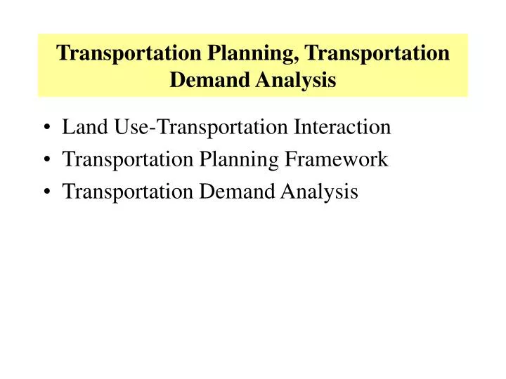
Transportation Planning, Transportation Demand Analysis. Land Use-Transportation Interaction Transportation Planning Framework Transportation Demand Analysis. Land Use-Transportation Interaction. Change in Land use. Transportation serves land uses. Change in Trip generation.

E N D
Transportation Planning, Transportation Demand Analysis • Land Use-Transportation Interaction • Transportation Planning Framework • Transportation Demand Analysis
Land Use-Transportation Interaction Change in Land use Transportation serves land uses Change in Trip generation Land Values Accessibility Change in travel needs Change in transportation supply (added services & facilities) Transportation shapes land uses
Land Use-Transportation-Environment Interaction Land use Transport Environment Urban Area . Zones . Change in land use over time (i.e. change in residential units, commercial land use, industrial land use, retail land use, etc.
Land Use Patterns, Bid Rent Pressure for growth Demand for land Bid rent Land use pattern Location of activities Bid rent $/sq.km CBD Distance from CBD Jobs Population Distance CBD
Purpose of Land Use Models • To explain/predict: Change in land use as a function of: - accessibility to employment - land value - percent of urban level available vacant land in a zone - public transit accessibility - quality of water & sewer services - etc..
Modelling Travel Decisions • User Decisions • 1. To travel (for a given trip purpose at a given time)? (Trip generation) • 2. Destination? (Trip distribution) • 3. Mode? (Modal Choice) • 4. Route? (Assignment of trip to network) • Modelling Approaches • Four-stage urban transportation modelling system (UTMS) • Unified approaches
Urban Transportation Demand Modelling: Four- Stage Modeling System Population & Employment Forecasts Trip Generation Trip Distribution Transportation Network & Service Attributes Modal Split Trip Assignment Link & O-D Flows, Times, Costs, Etc.
Four Stages of Urban Travel Demand Modelling I Trip Generation J Dj Oi Trip DistributionTij J I J Tij,auto I Mode Split J Tij, transit Traffic assignment I J Path of flowTij,auto through the auto network
Multiple Trip Purposes Population Employment Trip Rates, etc. HWHS NWS Generation Generation Generation Distribution Distribution Distribution Modal Split Modal Split Modal Split Road Assignment Transit Assignment Transport Network Link & O-D volumes, times, costs, v/c ratios, etc.
The Traffic Prediction Process Trip generation P & A Transit network Road network Trip distribution Modal split Transit person trips Auto person trips Occupancy Occupancy Transit vehicle trips Auto vehicle trips Freight & other vehicles Transit traffic assignment Road traffic assignment
Trip Generation • Modelling Methods • Linear regression method • Cross-classification (category analysis) method/trip rate method • _______________________________________________________ • Trip generation • Productions & Attractions • Home-based & non-home based • trips J I Zones
Trip Productions & Attractions Pi= Trip productions of zone i = f(land use, socio-economic characteristics of zone i) Aj= Attractions of zone j = f(land use, socio-economic characteristics of zone j) Regression Model Examples: (P.M. Peak Period Work Trips) Pi= 0.4572 emp - 138 (R2 = 0.87) Aj= 0.1848 pop + 9 (R2 = 0.90) Where emp is total employment pop is total population
Trip Productions & Attractions (Continued) Regression Model Examples: (P.M. Peak Period Non-work trips) Pi= 0.1346pop+0.2897emp+0.0043GLA (R2 = 0.76) Aj= 0.0888emp+ 0.6204DWEL+0.0045GLA+221 (R2 = 0.80) Where emp: is total employment pop: is total population GLA: shopping centre gross leasable area (ft2) DWEL: Dwelling units
Trip Productions & Attractions (Continued) RegressionModel Development Data Required Zone Pi*Aj*popempGLADWEL 1 …. .… …. …. …. ….. 2 …. .… …. …. …. ….. . _____________________________________________ * from O-D survey Data on other variables obtained from city data base
Trip Productions & Attractions (Continued) RegressionModel Development (Continued): Check on : - Partial correlation coefficient (r) . Should be high between P (the dependent variable) & other variables (the independent variables) & Should be high between A (the dependent variable) & other variables (the independent variables) . Should be low between pop, emp, GLA, DWEL (I.e. between independent variables) - Other statistical measures (“t” statistic for each independent variable)
Trip Productions & Attractions (Continued) RegressionModel Development (Continued): Check on : - R Multiple correlation coefficient (max. value of 1.0) - R2 Coefficient of multiple determination (max. value of 1.0) - Standard Error of Estimate (for the dependent variable - e.g. for Pi) Its value can be checked against the estimated values of the dependent variable. Example: A range of Pi values: 1,000-5,000; St. Error of 100 (very low!)
Trip Productions & Attractions (Continued) Trip Generation Rates (Cross Classification Approach) Trip Production: Step 1 Family Size Auto Ownership 0 1 2 or more 1 Trips/household/day 2 3 4 or more
Trip Productions & Attractions (Continued) Trip Generation Rates (Cross Classification Approach) Trip Production: Step 2 Trip productions for Zone i = (Trips/household/day) x (No. of households of that classification). Trips/household/day: is based on O-D survey No of households of a given classification: to be forecasted.
Trip Distribution Models Zone j Aj • Many models; most common is gravity model Zone i Pi Tij Zone j Aj Zone j Aj
Trip Distribution Models Aj Fij Kij Tij = Pi[ ] Origin-Constrained Gravity Model Σ for j(Aj Fij Kij) Where Tij = Trips produced in zone I and attracted to zone j Pi = Trips produced by zone i Aj = Trips attracted to zone j Fij = Impedance of travel from zone I to zone j (a travel time factor -- expressing an area-wide effect of distance) Kij = A zone-to -zone adjustment factor
Trip Distribution Models Pi Fij Kij Tij = Aj[ ] Destination-Constrained Gravity Model Σ for i(Pi Fij Kij) Where Tij = Trips produced in zone I and attracted to zone j Pi = Trips produced by zone i Aj = Trips attracted to zone j Fij = Impedance of travel from zone I to zone j (a travel time factor -- expressing an area-wide effect of distance) Kij = A zone-to -zone adjustment factor
Gravity Model The Fij is usually a some function of the travel time or generalized cost of travel between zones Fij = C-αij or Fij = t-αij Fij Where α is the calibration constant Fij = Travel time factor C ij = Generalized cost function t ij = Travel time Kij = A zone-to-zone adjustment factor (takes into account special characteristics of ij combinations tij or Cij Example River Zone 1 Zone 2
Gravity Model Note: Pi = Σ for j Tij Aj = Σ for i Tij Pi Aj
Gravity Model Example Using a gravity model with an impedance term of the form C-α , estimate the number of of trips from zone 1 to all other zones. α = 1.80. Other inputs are shown below. Zone Travel time to zone 1 (min) Productions Attractions 1 -- 5000 1000 2 10 2000 4000 3 20 4000 5000 4 15 3000 4000 __________________________________________________
Gravity Model Here, Pi for i = zone 1 are to be distributed to other zones by using the gravity model. Assume all K = 1 For α = 1.80 and given travel times Cij,, and Aj, we find: ______________________________________________ Zone Aj Cij C-α AjC- αij Tij 1 1000 -- -- -- -- 2 4000 10 1/63.1 63.40 2716* 3 5000 20 1/219.7 22.76 975 4 4000 15 1/130.91 30.56 1309 Sum 116.72 5000 * T from 1 to 2= 5000(63.40/116.72) = 2716
Gravity Model • Following iteration 1 of finding Tij from every zone to all zones, check to see if Ajsmatch the known values • If yes, the trip distribution problem is solved. • If not, the Ajshave to be adjusted. • The adjustment process is an iterative one (not covered here)