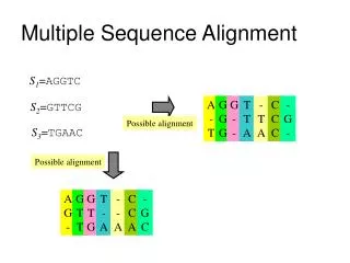
Download
1 / 40
410 likes | 615 Vues
Multiple sequence alignment and phylogenetic trees. Stat 246, Spring 2002, Week 5b. A version of the “tree of life”. Obtained from aligned sequences of ribosomal RNA. X. X. X. Y. Y. Y. Z. Z. Z. Species trees and gene trees (after M. Nei 1987, Molecular Evolutionary Genetics.).

E N D
Multiple sequence alignment and phylogenetic trees Stat 246, Spring 2002, Week 5b
A version of the “tree of life” Obtained from aligned sequences of ribosomal RNA
X X X Y Y Y Z Z Z Species trees and gene trees(after M. Nei 1987, Molecular Evolutionary Genetics.) Genes can be polymorphic before speciation, in different ways. Time A A A B B B
A E C D B F A E C D B F F B D C E A A E D C B F Tree topology Identical: Not identical:
Tree reconstruction A B A C B C C A B
A C B D B C A D C D A B D C A B A B C D B A C D C B A D A D C B B D C A C A B D D A B C A B C D A C B D A D B C Tree reconstruction (2) D B C A
Tree reconstruction (3) • In general, for any strictly bifurcating rooted tree with n species, there are • different topologies. • n#trees • 5 105 • 15 213,458,046,676,875 • 20 8,200,794,532,637,891,559,375 • For unrooted trees, it’s only
Tree reconstruction (4) • Distance-based methods • UPGMA • Transformed distance • Neighbors relation • Neighbor-joining • Character state-based methods • Maximum parsimony • Linear invariants • Maximum Likelihood
Beta-globins (orthologues) 10 20 30 40 BG-human M V H L T P E E K S A V T A L W G K V N V D E V G G E A L G R L L V V Y P W T Q BG-macaque - . . . . . . . . N . . . T . . . . . . . . . . . . . . . . . . . . . . . . . . BG-bovine - - M . . A . . . A . . . . F . . . . K . . . . . . . . . . . . . . . . . . . . BG-platypus - . . . S G G . . . . . . N . . . . . . I N . L . . . . . . . . . . . . . . . . BG-chicken . . . W . A . . . Q L I . G . . . . . . . A . C . A . . . A . . . I . . . . . . BG-shark - . . W S E V . L H E I . T T . K S I D K H S L . A K . . A . M F I . . . . . T 50 60 70 80 BG-human R F F E S F G D L S T P D A V M G N P K V K A H G K K V L G A F S D G L A H L D BG-macaque . . . . . . . . . . S . . . . . . . . . . . . . . . . . . . . . . . . . N . . . BG-bovine . . . . . . . . . . . A . . . . N . . . . . . . . . . . . D S . . N . M K . . . BG-platypus . . . . A . . . . . S A G . . . . . . . . . . . . A . . . T S . G . A . K N . . BG-chicken . . . A . . . N . . S . T . I L . . . M . R . . . . . . . T S . G . A V K N . . BG-shark . Y . G N L K E F T A C S Y G - - - - - . . E . A . . . T . . L G V A V T . . G 90 100 110 120 BG-human N L K G T F A T L S E L H C D K L H V D P E N F R L L G N V L V C V L A H H F G BG-macaque . . . . . . . Q . . . . . . . . . . . . . . . . K . . . . . . . . . . . . . . . BG-bovine D . . . . . . A . . . . . . . . . . . . . . . . K . . . . . . . V . . . R N . . BG-platypus D . . . . . . K . . . . . . . . . . . . . . . . N R . . . . . I V . . . R . . S BG-chicken . I . N . . S Q . . . . . . . . . . . . . . . . . . . . D I . I I . . . A . . S BG-shark D V . S Q . T D . . K K . A E E . . . . V . S . K . . A K C F . V E . G I L L K 130 140 BG-human K E F T P P V Q A A Y Q K V V A G V A N A L A H K Y H . means same as reference sequence - means deletion BG-macaque . . . . . Q . . . . . . . . . . . . . . . . . . . . . BG-bovine . . . . . V L . . D F . . . . . . . . . . . . . R . . BG-platypus . D . S . E . . . . W . . L . S . . . H . . G . . . . BG-chicken . D . . . E C . . . W . . L . R V . . H . . . R . . . BG-shark D K . A . Q T . . I W E . Y F G V . V D . I S K E . .
Beta-globins: Uncorrected pairwise distances Distances: between protein sequences. Calculated over: 1 to 147 Below diagonal: observed number of differences Above diagonal: number of differences per 100 amino acids hum mac bov pla chi sha hum ---- 5 16 23 31 65 mac 7 ---- 17 23 30 62 bov 23 24 ---- 27 37 65 pla 34 34 39 ---- 29 64 chi 45 44 52 42 ---- 61 sha 91 88 91 90 87 ----
Beta-globins: Corrected pairwise distances Distances: between protein sequences. Calculated over: residues 1 to 147 Below diagonal: observed number of differences Above diagonal: estimated number of substitutions per 100 amino acids Correction method: Jukes-Cantor (see Von Bing’s lecture) hum mac bov pla chi sha hum ---- 5 17 27 37 108 mac 7 ---- 18 27 36 102 bov 23 24 ---- 32 46 110 pla 34 34 39 ---- 34 106 chi 45 44 52 42 ---- 98 sha 91 88 91 90 87 ----
BG-shark BG-chicken BG-platypus BG-bovine BG-macaque BG-human UPGMA tree
UPGMA tree (alternate form) BG-shark BG-chicken BG-platypus BG-bovine BG-human BG-macaque
Human globins(paralogues) 10 20 30 alpha-human - V L S P A D K T N V K A A W G K V G A H A G E Y G A E A L E R M F L S F P T T beta-human V H . T . E E . S A . T . L . . . . - - N V D . V . G . . . G . L L V V Y . W . delta-human V H . T . E E . . A . N . L . . . . - - N V D A V . G . . . G . L L V V Y . W . epsilon-human V H F T A E E . A A . T S L . S . M - - N V E . A . G . . . G . L L V V Y . W . gamma-human G H F T E E . . A T I T S L . . . . - - N V E D A . G . T . G . L L V V Y . W . myo-human - G . . D G E W Q L . L N V . . . . E . D I P G H . Q . V . I . L . K G H . E . 40 50 60 70 alpha-human K T Y F P H F - D L S H G S A - - - - - Q V K G H G K K V A D A L T N A V A H V beta-human Q R F . E S . G . . . T P D . V M G N P K . . A . . . . . L G . F S D G L . . L delta-human Q R F . E S . G . . . S P D . V M G N P K . . A . . . . . L G . F S D G L . . L epsilon-human Q R F . D S . G N . . S P . . I L G N P K . . A . . . . . L T S F G D . I K N M gamma-human Q R F . D S . G N . . S A . . I M G N P K . . A . . . . . L T S . G D . I K . L myo-human L E K . D K . K H . K S E D E M K A S E D L . K . . A T . L T . . G G I L K K K 80 90 100 110 alpha-human D D M P N A L S A L S D L H A H K L R V D P V N F K L L S H C L L V T L A A H L beta-human . N L K G T F A T . . E . . C D . . H . . . E . . R . . G N V . V C V . . H . F delta-human . N L K G T F . Q . . E . . C D . . H . . . E . . R . . G N V . V C V . . R N F epsilon-human . N L K P . F A K . . E . . C D . . H . . . E . . . . . G N V M V I I . . T . F gamma-human . . L K G T F A Q . . E . . C D . . H . . . E . . . . . G N V . V T V . . I . F myo-human G H H E A E I K P . A Q S . . T . H K I P V K Y L E F I . E . I I Q V . Q S K H 120 130 140 alpha-human P A E F T P A V H A S L D K F L A S V S T V L T S K Y R - - - - - - beta-human G K . . . . P . Q . A Y Q . V V . G . A N A . A H . . H . . . . . . delta-human G K . . . . Q M Q . A Y Q . V V . G . A N A . A H . . H . . . . . . epsilon-human G K . . . . E . Q . A W Q . L V S A . A I A . A H . . H . . . . . . gamma-human G K . . . . E . Q . . W Q . M V T A . A S A . S . R . H . . . . . . myo-human . G D . G A D A Q G A M N . A . E L F R K D M A . N . K E L G F Q G
Human globins: uncorrected pairwise distances Distances: between protein sequences. Calculated over: 1 to 154 Below diagonal: observed number of differences Above diagonal: number of differences per 100 amino acids alpha beta delta eps gamma myo alpha ---- 55 55 60 57 74 beta 82 ---- 7 25 27 75 delta 82 10 ---- 27 29 74 Eps 89 35 39 ---- 20 77 gamma 85 39 42 29 ---- 76 myo 116 117 116 119 118 ----
Human globinsCorrected pairwise distances Distances: between protein sequences. Calculated over: 1 to 141 Below diagonal: observed number of differences Above diagonal: estimated number of substitutions per 100 amino acids Correction method: Jukes-Cantor alpha beta delta epsil gamma myo alpha ---- 281 281 281 313 208 beta 82 ---- 7 30 31 1000 delta 82 10 ---- 34 33 470 epsil 89 35 39 ---- 21 402 gamma 85 39 42 29 ---- 470 myo 116 117 116 119 118 ----
myo-human alpha-human epsilon-human gamma-human beta-human delta-human Neighbor-joining tree for globins
gamma-human epsilon-human alpha-human myo-human beta-human delta-human Neighbor-joining tree for globins (alternate form)
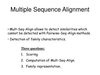
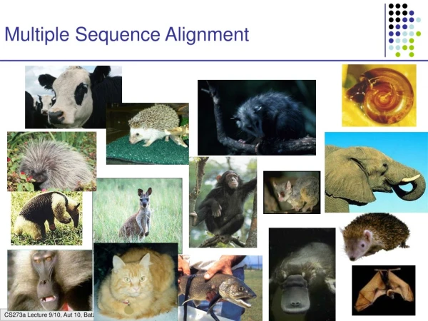
Why multiple alignment? • The simultaneous alignment of a number of DNA or protein sequences is one of the commonest tasks in bioinformatics. • Useful for: • phylogenetic analysis (inferring a tree, estimating rates of substitution, etc.) • detection of homology between a newly sequenced gene and an existing gene family • prediction of protein structure • demonstration of homology in multigene families • determination of a consensus sequence (e.g., in assembly)
Extending the pairwisealignment algorithms • Generally not feasible for more than a small number of sequences (~5), as the necessary computer time and space quickly becomes prohibitive. Computational time grows as Nm, where m = number of sequences. For example, for 100 residues from 5 species, 1005 = 10,000,000,000 (i.e., the equivalent of two sequences each 100,000 residues in length.) • Nor is it wholly desirable to reduce multiple alignment to a similar mathematical problem to that tackled by pairwise alignment algorithms. Two issues which are important in discussions of multiple alignment are: • the treatment of gaps: position-specific and/or residue-specific gap penalties are both desirable and feasible, and • the phylogenetic relationship between the sequences (which must exist if they are alignable): it should be exploited.
Progressive alignment Up until about 1987, multiple alignments would typically be constructed manually, although a few computer methods did exist. Around that time, algorithms based on the idea of progressive alignment appeared. In this approach, a pairwise alignment algorithm is used iteratively, first to align the most closely related pair of sequences, then the next most similar one to that pair, and so on. The rule “once a gap, always a gap” was implemented, on the grounds that the positions and lengths of gaps introduced between more similar pairs of sequences should not be affected by more distantly related ones.
Multiple alignment in 2002 The most widely used progressive alignment algorithm is currently CLUSTAL W. However, there are a number of more specialized procedures based on quite different principles, including the use of hidden Markov models built for protein families. A relatively new and promising approach uses Markov chain Monte Carlo methods to sample alignments according to certain probabilistic procedures and, by moving randomly around in the huge space of possible alignments, to find good alignments.
CLUSTAL W The three basic steps in the CLUSTAL W approach are shared by all progressive alignment algorithms: A. Calculate a matrix of pairwise distances based on pairwise alignments between the sequences B. Use the result of A to build a guide tree, which is an inferred phylogeny for the sequences C. Use the tree from B to guide the progressive alignment of the sequences
Calculating the pairwise distances (A) A pair of sequences is aligned by the usual dynamic programming algorithm, and then a similarity or distance measure for the pair is calculated using the aligned portion (gaps excluded) - for example, percent identity. CLUSTAL W does not correct these distances for multiple substitutions (e.g., by the Jukes-Cantor formula), although other programs do, and it is sometimes an option in different versions of the program.
Building the guide tree (B) • There are many ways of building a tree from a matrix of pairwise distances. CLUSTAL W uses the neighbour-joining (NJ) method, which is the most favoured approach these days. Earlier versions of CLUSTAL used the unweighted pair group method usingarithmetic averages (UPGMA), and this is still used in some programs. • A root of the tree is then determined by the so-called mid-point method (giving equal means for the branch lengths on either side of the root). • The W in CLUSTAL W stands for Weights, an important feature of this program. These are calculated in a straightforward way. They correct for unequal sampling at different evolutionary distances.
myg_phyca lgb2_luplu glb5_petma hba_human hba_horse hbb_horse hbb_human NJ globin tree
Tree, distances, and weightsThompson et al. (1994) .081 hbb human: 0.221 .226 .084 hbb horse: 0.225 .061 .055 hba human: 0.194 .219 .015 .065 hba horse: 0.203 .062 .398 myg phyca: 0.411 .389 glb5 petma: 0.398 .442 lgb2 luplu: 0.442
Progressive alignment (C) The basic idea is to use a series of pairwise alignments to align larger and larger groups of sequences, following the branching order of the guide tree. We proceed from the tips of the rooted tree towards the root. In our globin example, we align in the following order: a) human and horse -globin; b) human and horse -globin; c) the two -globins and the two -globins; d) myoglobin and the haemoglobins; e) cyanohaemoglobin and the combined haemoglobin, myoglobin group; f) leghaemoglobin and the rest.
Progressive alignment (C, 2) At each stage a full dynamic programming algorithm is used, with a residue scoring matrix (e.g., a PAM or a BLOSUM matrix) and gap opening and extension penalties. Each step consists of aligning two existing alignments. Scores at a position are averages of all pairwise scores for residues in the two sets of sequences using matrices with only positive values. Gap vs. residue scores zero. Sequence weights are used at this stage. See next slide. Gaps that are present in older alignments remain fixed. New gaps introduced at each stage initially get full opening and extension penalties, even if inside old gap positions. This gets modified.
1 peeksavtal 2 geekaavlal 3 padktnvkaa 4 aadktnvkaa 5 egewqlvlhv 6 aaektkirsa Sequence weights w1,...,w6 Score: Scoring an alignment of two partial alignments
Progressive alignment (C) - gaps CLUSTAL W has quite a sophisticated treatment of gaps, incorporating into opening and extension penalties a dependence on a) weight matrix, b) sequence similarity, c) sequence length, d) difference in sequence length, e) position of gaps (see figure), f) residues at gaps. Regarding e) and f), the motivation is as follows: if one knew the positions of all secondary structure elements (-helices, -strands) in all or some of the sequences, one could increase the gap penalties inside and decrease outside them, forcing gaps to occur most often in loop regions, which is what is observed in alignments of sequences with known 3-D structure. For further details, see Thompson et al., NAR 1994, 22:4673 or Methods in Enz. 1996, 266:article 22.
Final CLUSTALW alignment (using eclustalw) 7 -helices
Alignment using Hidden Markov models There are now many HMMs for protein families such as globins, and these models can be used to infer alignments of new globin sequences to other members of the family. Such models can also be used to determine whether a given sequence is or is not a member of a specified family.
Web-based multiple sequence alignment • ClustalW • www2.ebi.ac.uk/clustalw/ • dot.imgen.bcm.tmc.edu:9331/multi-align/Options/clustalw.html • www.clustalw.genome.ad.jp/ • bioweb.pasteur.fr/intro-uk.html • pbil.ibcp.fr • transfac.gbf.de/programs.html • www.bionavigator.com • PileUp • helix.nih.gov/newhelix • www.hgmp.mrc.ac.uk/ • bcf.arl.arizona.edu/gcg.html • www.bionavigator.com • Dialign • genomatix.gsf.de/ • bibiserv.techfak.uni-bielefeld.de/ • bioweb.pasteur.fr/intro-uk.html • www.hgmp.mrc.ac.uk/ • Match-box • www.fundp.ac.be/sciences/biologie/bms/matchbox_submit.html • For reviews: G. J. Gaskell, BioTechniques 2000, 29:60, and • www.techfak.uni-bielefeld.de/bcd/Curric/MulAli/welcome.html
Comparing multiple sequence alignment programs • Even below the 10-20% identity twilight zone, the best programs correctly align 47% of residues on average • Iterative algorithms are superior, but with a large trade-off in use of computational resources • Global generally performs better than local • No single ‘best’ program exists • For reviews, see: • P. Briffeuil et al., Bioinformatics 1998, 14:357 • J. D. Thompson et al., NAR 1999, 27:2682
Multiple sequence alignment editors • EditSeq/MegAlign - Lasergene - Mac or MS-Windows • DNA Strider - Macintosh • Seq-Al - Macintosh • ASAD - Excel - Macintosh or MS-Windows • BioEdit - MS-Windows • Genedoc - MS-Windows • SeqPup - Mac. MS-Windows, X-Windows • For a review of these: http://www.wehi.edu.au/bioweb/KeithsStuff/seqeditors.html