Download
1 / 73
730 likes | 1.15k Vues
Parallel Spectral Methods: Fast Fourier Transform (FFTs) with Applications. James Demmel www.cs.berkeley.edu/~demmel/cs267_Spr10. Motifs. The Motifs (formerly “Dwarfs”) from “The Berkeley View” ( Asanovic et al.) Motifs form key computational patterns. Topic of this lecture. 2.

E N D
Parallel Spectral Methods:Fast Fourier Transform (FFTs)with Applications James Demmel www.cs.berkeley.edu/~demmel/cs267_Spr10 CS267 Lecture 20
Motifs The Motifs (formerly “Dwarfs”) from “The Berkeley View” (Asanovic et al.) Motifs form key computational patterns Topic of this lecture CS267 Lecture 21 2
Ouline and References • Outline • Definitions • A few applications of FFTs • Sequential algorithm • Parallel 1D FFT • Parallel 3D FFT • Autotuning FFTs: FFTW and Spiral projects • References • Previous CS267 lectures • FFTW project: http://www.fftw.org • Spiral project: http://www.spiral.net • Lecture by Geoffrey Fox: http://grids.ucs.indiana.edu/ptliupages/presentations/PC2007/cps615fft00.ppt CS267 Lecture 20
Definition of Discrete Fourier Transform (DFT) • Let i=sqrt(-1) and index matrices and vectors from 0. • The (1D) DFT of an m-element vector v is: • F*v • where F is an m-by-m matrix defined as: • F[j,k] = v(j*k) • and where v is: • v = e (2pi/m) = cos(2p/m) + i*sin(2p/m) • v is a complex number with whose mthpower vm =1 and is therefore called an mth root of unity • E.g., for m = 4: v = i, v2 = -1, v3 = -i, v4 = 1 • The 2D DFT of an m-by-m matrix V is F*V*F • Do 1D DFT on all the columns independently, then all the rows • Higher dimensional DFTs are analogous CS267 Lecture 20
Motivation for Fast Fourier Transform (FFT) • Signal processing • Image processing • Solving Poisson’s Equation nearly optimally • O(n log n) arithmetic operations • Fast multiplication of large integers • … CS267 Lecture 21
Using the 1D FFT for filtering • Signal = sin(7t) + .5 sin(5t) at 128 points • Noise = random number bounded by .75 • Filter by zeroing out FFT components < .25 CS267 Lecture 21
Using the 2D FFT for image compression • Image = 200x320 matrix of values • Compress by keeping largest 2.5% of FFT components • Similar idea used by jpeg CS267 Lecture 20
Recall: Poisson’s equation arises in many models 3D: 2u/x2 + 2u/y2 + 2u/z2 = f(x,y,z) • Electrostatic or Gravitational Potential: Potential(position) • Heat flow: Temperature(position, time) • Diffusion: Concentration(position, time) • Fluid flow: Velocity,Pressure,Density(position,time) • Elasticity: Stress,Strain(position,time) • Variations of Poisson have variable coefficients f represents the sources; also need boundary conditions 2D: 2u/x2 + 2u/y2 = f(x,y) 1D: d2u/dx2 = f(x) CS267 Lecture 20
Solving Poisson Equation with FFT (1/2) Graph and “5 pointstencil” Graph and “stencil” 4 -1 -1 -1 4 -1 -1 -1 4 -1 -1 4 -1 -1 -1 -1 4 -1 -1 -1 -1 4 -1 -1 4 -1 -1 -1 4 -1 -1 -1 4 -1 -1 2 -1 -1 4 -1 L2= • 2D Poisson equation: solve L2x = b where -1 2 -1 -1 2 -1 -1 2 -1 -1 2 -1 -1 2 3D case is analogous (7 point stencil) L1 = 1D Poisson equation: solve L1x = b where CS267 Lecture 21
Solving 2D Poisson Equation with FFT (2/2) • Use facts that • L1 = F · D · FT is eigenvalue/eigenvector decomposition, where • F is very similar to FFT (imaginary part) • F(j,k) = (2/(n+1))1/2 · sin(j k /(n+1)) • D = diagonal matrix of eigenvalues • D(j,j) = 2(1 – cos(j / (n+1)) ) • 2D Poisson same as solving L1 · X + X · L1 = B where • X square matrix of unknowns at each grid point, B square too • Substitute L1 = F · D · FT into 2D Poisson to get algorithm • Perform 2D “FFT” on B to get B’ = FT ·B · F • Solve D X’ + X’ D = B’ for X’: X’(j,k) = B’(j,k)/ (D(j,j) + D(k,k)) • Perform inverse 2D “FFT” on X’ to get X: get X = F ·X’ · FT • Cost = 2 2D-FFTs plus n2 adds, divisions • 3D Poisson analogous CS267 Lecture 20
Algorithms for 2D (3D) Poisson Equation (N = n2(n3) vars) Algorithm Serial PRAM Memory #Procs • Dense LU N3 N N2 N2 • Band LU N2 (N7/3) N N3/2 (N5/3) N (N4/3) • Jacobi N2 (N5/3) N (N2/3) N N • Explicit Inv. N2 log N N2 N2 • Conj.Gradients N3/2 (N4/3) N1/2(1/3) *log N N N • Red/Black SOR N3/2 (N4/3) N1/2 (N1/3) N N • Sparse LU N3/2 (N2)N1/2 N*log N (N4/3) N • FFT N*log N log N N N • Multigrid N log2 N N N • Lower bound N log N N PRAM is an idealized parallel model with zero cost communication Reference: James Demmel, Applied Numerical Linear Algebra, SIAM, 1997. CS267 Lecture 20
Related Transforms • Most applications require multiplication by both F and F-1 • Multiplying by F and F-1 are essentially the same. • F-1 = complex_conjugate(F) / n • For solving the Poisson equation and various other applications, we use variations on the FFT • The sin transform -- imaginary part of F • The cos transform -- real part of F • Algorithms are similar, so we will focus on F. CS267 Lecture 20
Serial Algorithm for the FFT • Compute the FFT (F*v) of an m-element vector v (F*v)[j] = S F(j,k) * v(k) = Sv(j*k) * v(k) = S (vj)k * v(k) = V(v j) where V is defined as the polynomial V(x) = S xk * v(k) m-1 k = 0 m-1 k = 0 m-1 k = 0 m-1 k = 0 CS267 Lecture 20
Divide and Conquer FFT • V can be evaluated using divide-and-conquer V(x) = S xk * v(k) = v[0] + x2*v[2] + x4*v[4] + … + x*(v[1] + x2*v[3] + x4*v[5] + … ) = Veven(x2) + x*Vodd(x2) • V has degree m-1, so Veven and Vodd are polynomials of degree m/2-1 • We evaluate these at m points: (v j)2 for 0 ≤ j ≤ m-1 • But this is really just m/2 different points, since (v(j+m/2) )2 = (vj *v m/2) )2 = v2j *v m = (vj)2 • So FFT on m points reduced to 2 FFTs on m/2 points • Divide and conquer! m-1 k = 0 CS267 Lecture 20
Divide-and-Conquer FFT (D&C FFT) FFT(v, v, m) if m = 1 return v[0] else veven = FFT(v[0:2:m-2], v 2, m/2) vodd = FFT(v[1:2:m-1], v 2, m/2) v-vec = [v0, v1, … v(m/2-1) ] return [veven + (v-vec .* vodd), veven - (v-vec .* vodd) ] • Matlab notation: “.*” means component-wise multiply. Cost: T(m) = 2T(m/2)+O(m) = O(m log m) operations. precomputed CS267 Lecture 20
An Iterative Algorithm • The call tree of the D&C FFT algorithm is a complete binary tree of log m levels • An iterative algorithm that uses loops rather than recursion, goes each level in the tree starting at the bottom • Algorithm overwrites v[i] by (F*v)[bitreverse(i)] • Practical algorithms combine recursion (for memory hierarchy) and iteration (to avoid function call overhead) – more later FFT(0,1,2,3,…,15) = FFT(xxxx) even odd FFT(0,2,…,14) = FFT(xxx0) FFT(1,3,…,15) = FFT(xxx1) FFT(xx00) FFT(xx10) FFT(xx01) FFT(xx11) FFT(x000) FFT(x100) FFT(x010) FFT(x110) FFT(x001) FFT(x101) FFT(x011) FFT(x111) FFT(0) FFT(8) FFT(4) FFT(12) FFT(2) FFT(10) FFT(6) FFT(14) FFT(1) FFT(9) FFT(5) FFT(13) FFT(3) FFT(11) FFT(7) FFT(15) CS267 Lecture 20
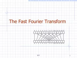
Parallel 1D FFT • Data dependencies in 1D FFT • Butterfly pattern • From veven w .* vodd • A PRAM algorithm takes O(log m) time • each step to right is parallel • there are log m steps • What about communication cost? • (See UCB EECS Tech report UCB/CSD-92-713 for details, aka “LogP paper”) CS267 Lecture 20
Block Layout of 1D FFT • Using a block layout (m/p contiguous elts per processor) • No communication in last log m/p steps • Each step requires fine-grained communication in first log p steps CS267 Lecture 20
Cyclic Layout of 1D FFT • Cyclic layout (only 1 element per processor, wrapped) • No communication in first log(m/p) steps • Communication in last log(p) steps CS267 Lecture 20
Parallel Complexity • m = vector size, p = number of processors • f = time per flop = 1 • a = latency for message • b = time per word in a message • Time(block_FFT) = Time(cyclic_FFT) = 2*m*log(m)/p … perfectly parallel flops + log(p) * a ... 1 message/stage, log p stages + m*log(p)/p * b … m/p words/message CS267 Lecture 20
FFT With “Transpose” • If we start with a cyclic layout for first log(p) steps, there is no communication • Then transpose the vector for last log(m/p) steps • All communication is in the transpose • Note: This example has log(m/p) = log(p) • If log(m/p) > log(p) more phases/layouts will be needed • We will work with this assumption for simplicity CS267 Lecture 20
Why is the Communication Step Called a Transpose? • Analogous to transposing an array • View as a 2D array of n/p by p • Note: same idea is useful for caches CS267 Lecture 20
Complexity of the FFT with Transpose • If no communication is pipelined (overestimate!) • Time(transposeFFT) = • 2*m*log(m)/p same as before • + (p-1) * a was log(p) * a • + m*(p-1)/p2 * b was m* log(p)/p* b • If communication is pipelined, so we do not pay for p-1 messages, the second term becomes simply a, rather than (p-1)a • This is close to optimal. See LogP paper for details. • See also following papers • A. Sahai, “Hiding Communication Costs in Bandwidth Limited FFT” • R. Nishtala et al, “Optimizing bandwidth limited problems using one-sided communication” CS267 Lecture 20
Comment on the 1D Parallel FFT • The above algorithm leaves data in bit-reversed order • Some applications can use it this way, like Poisson • Others require another transpose-like operation • Other parallel algorithms also exist • A very different 1D FFT is due to Edelman (see http://www-math.mit.edu/~edelman) • Based on the Fast Multipole algorithm • Less communication for non-bit-reversed algorithm CS267 Lecture 20
Higher Dimensional FFTs • FFTs on 2 or more dimensions are defined as 1D FFTs on vectors in all dimensions. • 2D FFT does 1D FFTs on all rows and then all columns • There are 3 obvious possibilities for the 2D FFT: • (1) 2D blocked layout for matrix, using parallel 1D FFTs for each row and column • (2) Block row layout for matrix, using serial 1D FFTs on rows, followed by a transpose, then more serial 1D FFTs • (3) Block row layout for matrix, using serial 1D FFTs on rows, followed by parallel 1D FFTs on columns • Option 2 is best, if we overlap communication and computation • For a 3D FFT the options are similar • 2 phases done with serial FFTs, followed by a transpose for 3rd • can overlap communication with 2nd phase in practice CS267 Lecture 20
Bisection Bandwidth • FFT requires one (or more) transpose operations: • Every processor sends 1/P of its data to each other one • Bisection Bandwidth limits this performance • Bisection bandwidth is the bandwidth across the narrowest part of the network • Important in global transpose operations, all-to-all, etc. • “Full bisection bandwidth” is expensive • Fraction of machine cost in the network is increasing • Fat-tree and full crossbar topologies may be too expensive • Especially on machines with 100K and more processors • SMP clusters often limit bandwidth at the node level • Goal: overlap communication and computation CS267 Lecture 20
LogGP: no overlap P0 osend L orecv P1 Modified LogGP Model • LogGP: no overlap P0 g P1 EEL: end to end latency (1/2 roundtrip) g: minimum time between small message sends G: additional gap per byte for larger messages CS267 Lecture 20
Historical Perspective ½ round-trip latency • Potential performance advantage for fine-grained, one-sided programs • Potential productivity advantage for irregular applications CS267 Lecture 20
General Observations • The overlap potential is the difference between the gap and overhead • No potential if CPU is tied up throughout message send • E.g., no send-side DMA • Potential grows with message size for machines with DMA (per byte cost is handled by network, i.e. NIC) • Potential grows with amount of network congestion • Because gap grows as network becomes saturated • Remote overhead is 0 for machine with RDMA CS267 Lecture 20
GASNet Communications System GASNet offers put/get communication • One-sided: no remote CPU involvement required in API (key difference with MPI) • Message contains remote address • No need to match with a receive • No implicit ordering required Compiler-generated code • Used in language runtimes (UPC, etc.) • Fine-grained and bulk transfers • Split-phase communication Language-specific runtime GASNet Network Hardware CS267 Lecture 20
Performance of 1-Sided vs 2-sided Communication: GASNet vs MPI • Comparison on Opteron/InfiniBand – GASNet’s vapi-conduit and OSU MPI 0.9.5 • Up to large message size (> 256 Kb), GASNet provides up to 2.2X improvement in streaming bandwidth • Half power point (N/2) differs by one order of magnitude CS267 Lecture 20
(up is good) GASNet: Performance for mid-range message sizes GASNet usually reaches saturation bandwidth before MPI - fewer costs to amortize Usually outperforms MPI at medium message sizes - often by a large margin CS267 Lecture 20
NAS FT Benchmark Case Study • Performance of Exchange (Alltoall) is critical • Communication to computation ratio increases with faster, more optimized 1-D FFTs (used best available, from FFTW) • Determined by available bisection bandwidth • Between 30-40% of the applications total runtime • Assumptions • 1D partition of 3D grid (a limitation) • At most N processors for N^3 grid • HPC Challenge benchmark has large 1D FFT (can be viewed as 3D or more with proper roots of unity) • Reference for details • “Optimizing Bandwidth Limited Problems Using One-side Communication and Overlap”, C. Bell, D. Bonachea, R. Nishtala, K. Yelick, IPDPS’06 (www.eecs.berkeley.edu/~rajashn) • Started as CS267 project CS267 Lecture 20
Performing a 3D FFT • NX x NY x NZ elements spread across P processors • Will Use 1-Dimensional Layout in Z dimension • Each processor gets NZ / P “planes” of NX x NY elements per plane Example: P = 4 NZ NZ/P 1D Partition NX p3 p2 p1 NY p0 Source: R. Nishtala, C. Bell, D. Bonachea, K. Yelick
Performing a 3D FFT (part 2) • Perform an FFT in all three dimensions • With 1D layout, 2 out of the 3 dimensions are local while the last Z dimension is distributed Step 1: FFTs on the columns (all elements local) Step 2: FFTs on the rows (all elements local) Step 3: FFTs in the Z-dimension (requires communication) Source: R. Nishtala, C. Bell, D. Bonachea, K. Yelick
Performing the 3D FFT (part 3) • Can perform Steps 1 and 2 since all the data is available without communication • Perform a Global Transpose of the cube • Allows step 3 to continue Transpose Source: R. Nishtala, C. Bell, D. Bonachea, K. Yelick
The Transpose • Each processor has to scatter input domain to other processors • Every processor divides its portion of the domain into P pieces • Send each of the P pieces to a different processor • Three different ways to break it up the messages • Packed Slabs (i.e. single packed “Alltoall” in MPI parlance) • Slabs • Pencils • Going from approach Packed Slabs to Slabs to Pencils leads to • An order of magnitude increase in the number of messages • An order of magnitude decrease in the size of each message • Why do this? Slabs and Pencils allow overlapping communication and computation and leverage RDMA support in modern networks Source: R. Nishtala, C. Bell, D. Bonachea, K. Yelick
Algorithm 1: Packed Slabs Example with P=4, NX=NY=NZ=16 • Perform all row and column FFTs • Perform local transpose • data destined to a remote processor are grouped together • Perform P puts of the data put to proc 0 put to proc 1 put to proc 2 put to proc 3 Local transpose • For 5123 grid across 64 processors • Send 64 messages of 512kB each Source: R. Nishtala, C. Bell, D. Bonachea, K. Yelick
Bandwidth Utilization • NAS FT (Class D) with 256 processors on Opteron/InfiniBand • Each processor sends 256 messages of 512kBytes • Global Transpose (i.e. all to all exchange) only achieves 67% of peak point-to-point bidirectional bandwidth • Many factors could cause this slowdown • Network contention • Number of processors with which each processor communicates • Can we do better? Source: R. Nishtala, C. Bell, D. Bonachea, K. Yelick
put to proc 0 put to proc 1 put to proc 2 put to proc 3 Algorithm 2: Slabs • Waiting to send all data in one phase bunches up communication events • Algorithm Sketch • for each of the NZ/P planes • Perform all column FFTs • for each of the P “slabs” (a slab is NX/P rows) • Perform FFTs on the rows in the slab • Initiate 1-sided put of the slab • Wait for all puts to finish • Barrier • Non-blocking RDMA puts allow data movement to be overlapped with computation. • Puts are spaced apart by the amount of time to perform FFTs on NX/P rows plane 0 Start computation for next plane • For 5123 grid across 64 processors • Send 512 messages of 64kB each Source: R. Nishtala, C. Bell, D. Bonachea, K. Yelick
1 3 2 2 2 2 1 1 3 0 0 0 0 3 3 1 Algorithm 3: Pencils • Further reduce the granularity of communication • Send a row (pencil) as soon as it is ready • Algorithm Sketch • For each of the NZ/P planes • Perform all 16 column FFTs • For r=0; r<NX/P; r++ • For each slab s in the plane • Perform FFT on row r of slab s • Initiate 1-sided put of row r • Wait for all puts to finish • Barrier • Large increase in message count • Communication events finely diffused through computation • Maximum amount of overlap • Communication starts early plane 0 Start computation for next plane • For 5123 grid across 64 processors • Send 4096 messages of 8kB each Source: R. Nishtala, C. Bell, D. Bonachea, K. Yelick
GASNet achieves close to peak bandwidth with Pencils but MPI is about 50% less efficient at 8k With the message sizes in Packed Slabs both comm systems reach the same peak bandwidth Communication Requirements With Slabs GASNet is slightly faster than MPI • 5123 across 64 processors • Alg 1: Packed Slabs • Send 64 messages of 512kB • Alg 2: Slabs • Send 512 messages of 64kB • Alg 3: Pencils • Send 4096 messages of 8kB Source: R. Nishtala, C. Bell, D. Bonachea, K. Yelick
Platforms Source: R. Nishtala, C. Bell, D. Bonachea, K. Yelick
Comparison of Algorithms • Compare 3 algorithms against original NAS FT • All versions including Fortran use FFTW for local 1D FFTs • Largest class that fit in the memory (usually class D) • All UPC flavors outperform original Fortran/MPI implantation by at least 20% • One-sided semantics allow even exchange based implementations to improve over MPI implementations • Overlap algorithms spread the messages out, easing the bottlenecks • ~1.9x speedup in the best case up is good Source: R. Nishtala, C. Bell, D. Bonachea, K. Yelick
Time Spent in Communication • Implemented the 3 algorithms in MPI using Irecvs and Isends • Compare time spent initiating or waiting for communication to finish • UPC consistently spends less time in communication than its MPI counterpart • MPI unable to handle pencils algorithm in some cases 28.6 312.8 34.1 MPI Crash (Pencils) down is good Source: R. Nishtala, C. Bell, D. Bonachea, K. Yelick
Performance Summary up is good Source: R. Nishtala, C. Bell, D. Bonachea, K. Yelick
FFTW – Fastest Fourier Transform in the West • www.fftw.org • Produces FFT implementation optimized for • Your version of FFT (complex, real,…) • Your value of n (arbitrary, possibly prime) • Your architecture • Very good sequential performance (competes with Spiral) • Similar in spirit to PHIPAC/ATLAS/OSKI/Sparsity • Won 1999 Wilkinson Prize for Numerical Software • Widely used for serial FFTs • Had parallel FFTs in version 2, but no longer supporting them (?) • Layout constraints from users/apps + network differences are hard to support CS267 Lecture 20
free software:http://www.fftw.org/ the “Fastest Fourier Tranform in the West” FFTW • C library for real & complex FFTs (arbitrary size/dimensionality) (+ parallel versions for threads & MPI) • Computational kernels (80% of code) automatically generated • Self-optimizes for your hardware (picks best composition of steps) = portability + performance CS267 Lecture 20
FFTW performancepower-of-two sizes, double precision 833 MHz Alpha EV6 2 GHz PowerPC G5 500 MHz Ultrasparc IIe 2 GHz AMD Opteron CS267 Lecture 21
FFTW performancenon-power-of-two sizes, double precision unusual: non-power-of-two sizes receive as much optimization as powers of two 833 MHz Alpha EV6 2 GHz AMD Opteron …because we let the code do the optimizing CS267 Lecture 20