Download
1 / 29
300 likes | 481 Vues
Prefiltered Single Scattering. Oliver Klehm , MPI Informatik Hans-Peter Seidel, MPI Informatik Elmar Eisemann , TU Delft. Motivation. Photo by Frédo Durand. near. Shadow Map. far. Assumptions: Single scattering. Shadow Map. Assumptions: Single scattering Homogeneous medium.

E N D
Prefiltered Single Scattering Oliver Klehm, MPI Informatik Hans-Peter Seidel, MPI Informatik ElmarEisemann, TU Delft
Motivation Photo by Frédo Durand
near Shadow Map far
Assumptions: • Single scattering
Shadow Map Assumptions: • Single scattering • Homogeneous medium
Shadow Map How to do this efficiently? Naïve: O(w*h * d) w*h pixels, d integration steps
Link to Percentage Closer Filtering Percentage Closer Filtering Light direction V(d,zS) Visibility function V
Shadow Mapping Light direction 0 p z Shadow Map d(x') z(p) Visibility function V(d,z) 1 d(x) 0 1 -1 -1 0 1 d(x')-z(p) x
Convolution Shadow Maps Approximate visibility function with truncated Fourier series V(d,z) V(d,z) a1 +a2 +..+a4 +..+a8 +..+a16 [Annen et al. 2007]
Convolution Shadow Maps Filtering s s V(d,z) = ai(d) Bi(z) Shadow Map z (1+1+0+0+0) 0 V(d,z) = s d
Convolution Shadow Maps Filtering • Compute Bi(zs) • Filter Bi • Compute ai(d) • Fetch filtered Bi , compute aiBi Only depends on depths in SM s s V(d,z) = ai(d) Bi(z) Shadow Map Filtering without knowledge of shading point! d At shading time
Filtering for camera rays V(d,z) = ai(d) Bi(z) s s BiMaps Filter Kernel Shadow Map S = 1 N d(constant for entire ray) camera ray
Filtering for camera rays V(d,z) = ai(d) Bi(z) s s Shadow Map BiMaps N? camera ray camera ray
Prefix Sum-like Filtering BiMap Filtered BiMap camera ray camera ray
Filtering for camera rays V(d,zS) = ai(dS) Bi(zS) Shadow Map d2 d7 d11 d16 d21
Rectified Shadow Map Light direction
Rectified Shadow Map Light direction
Rectified Shadow Map Light direction
Rectified Shadow Map Light direction
Related Work • Complexity:(w*h pixels, d*a shadow map, allowing for d marching-steps) • Ray-marching: O(w*h * d) • Tree-based structures on rectified shadow map • [Baran et al. 2010] “A hierarchical volumetric shadow algorithm for single scattering” • [Chen et al. 2011] “Realtime volumetric shadows using 1d min-max mipmaps” • Tree average: O(w*h * log d + a*d) • Tree worst: O(w*h * d + a*d) • Ours: O(w*h * C + C * a*d )(C basis functions) O(w*h + a*d)
Limitations • Light dependent falloff functions • Local light sources • Degenerated cases of perspective projection • Ringing artifacts (similar to convolution shadow maps)
Limitations • Ringing artifacts (similar to convolution shadow maps)
Nitty Gritty Details (in the paper) • Not average visibility, but medium attenuation? • Add weights to filtering • Other visibility linearization methods? • Exponential shadow maps • Variance shadow maps • Exponential variance shadow maps • Fast prefix-sum-like filtering?
Conclusions • Volumetric single scattering - constant time per pixel • Purely image-based, no scene dependence • New light projection for rectified shadow map • Fast, high-quality effects 2.2 ms 30 fps