Download

1 / 25
250 likes | 397 Vues
Chapter 5 Linear Inequalities and Linear Programming. Section 3 Linear Programming in Two Dimensions: A Geometric Approach. Learning Objectives for Section 5.3. Linear Programming in Two Dimensions: Geometric Approach.

E N D
Chapter 5Linear Inequalities and Linear Programming Section 3 Linear Programming in Two Dimensions: A Geometric Approach
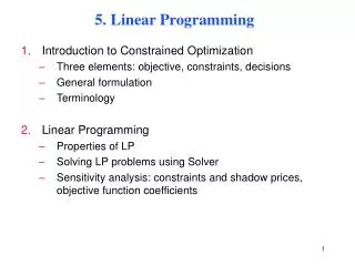
Learning Objectives for Section 5.3 Linear Programming in Two Dimensions: Geometric Approach • The student will be able to set up decision variables and formulate a linear programming problem. • The student will be able to solve linear programming problems using a geometric approach. • The student will be able to solve applications using linear programming methods. Barnett/Ziegler/Byleen Finite Mathematics 12e
Linear Programming in Two Dimensions: A Geometric Approach In this section, we will explore applications which utilize the graph of a system of linear inequalities. Barnett/Ziegler/Byleen Finite Mathematics 12e
A Familiar Example We have seen this problem before. An extra condition will be added to make the example more interesting. Suppose a manufacturer makes two types of skis: a trick ski and a slalom ski. Each trick ski requires 8 hours of design work and 4 hours of finishing. Each slalom ski requires 8 hours of design and 12 hours of finishing. Furthermore, the total number of hours allocated for design work is 160 and the total available hours for finishing work is 180. Finally, the number of trick skis produced must be less than or equal to 15. How many trick skis and how many slalom skis can be made under these conditions? Now, here is the twist: Suppose the profit on each trick ski is $5 and the profit for each slalom ski is $10. How many each of each type of ski should the manufacturer produce to earn the greatest profit? Barnett/Ziegler/Byleen Finite Mathematics 12e
Linear Programming Problem This is an example of a linear programming problem. Every linear programming problem has two components: 1. A linear objective function is to be maximized or minimized. In our case the objective function is Profit = 5x + 10y (5 dollars profit for each trick ski manufactured and $10 for every slalom ski produced). 2. A collection of linear inequalities that must be satisfied simultaneously. These are called the constraints of the problem because these inequalities give limitations on the values of xand y. In our case, the linear inequalities are the constraints. Barnett/Ziegler/Byleen Finite Mathematics 12e
Constraints x and y have to be positive The number of trick skis must be less than or equal to 15 Design constraint: 8 hours to design each trick ski and 8 hours to design each slalom ski. Finishing constraint: 4 hours for each trick ski and 12 hours for each slalom ski. Barnett/Ziegler/Byleen Finite Mathematics 12e
Linear Programming Problem(continued) 3. The feasible set is the set of all points that are possible solutions. In this case, we want to determine the value(s) of x, the number of trick skis and y, the number of slalom skis that will yield the maximum profit. Only certain points are eligible. Those are the points within the common region of intersection of the graphs of the constraining inequalities. Let’s return to the graph of the system of linear inequalities. Notice that the feasible set is the yellow shaded region. Our task is to maximize the profit function P = 5x + 10y by producing x trick skis and y slalom skis, but use only values of x and y that are within the yellow region graphed in the next slide. Barnett/Ziegler/Byleen Finite Mathematics 12e
The Feasible Set Barnett/Ziegler/Byleen Finite Mathematics 12e
Maximizing the Profit The profit is given by P = 5x + 10y. The equation k = 5x + 10y represents a line with slope (-1/2). For each point (x, y) on this line, the profit equals k. This is called an constant-profit line. As the profit k increases, the line shifts upward by the amount of increase while remaining parallel to all other constant-profit lines. What we are attempting to do is to find the largest value of k possible. The graph on the next slide shows a few isoprofit lines. The maximum value of profit occurs at a corner point - a point of intersection of two lines. Barnett/Ziegler/Byleen Finite Mathematics 12e
Constant-profit Lines The exact point of intersection of the two lines is (7.5,12.5). Since x and y must be whole numbers, we round the answer down to (7,12). Barnett/Ziegler/Byleen Finite Mathematics 12e
Maximizing the Profit(continued) The maximum value of the profit function in this example was at the corner point, (7.5, 12.5), but since we cannot produce a fraction of a ski, we will round down to (7, 12). We cannot exceed the constraints, so we can’t round up. Thus, the manufacturer should produce 7 trick skis and 12 slalom skis to achieve maximum profit. What is the maximum profit? P = 5x + 10y P = 5(7)+10(12) = 35 + 120 = 155. Barnett/Ziegler/Byleen Finite Mathematics 12e
General Result • If a linear programming problem has a solution, it is located at a corner point of the set of feasible solutions. If a linear programming problem has more than one solution, at least one of them is located at a corner point of the set of feasible solutions. • If the set of feasible solutions is bounded, as in our example, the solution of the linear programming problem will exist. Bounded means that the region can be enclosed in a circle. • If the set of feasible solutions is not bounded, then the solution may or may not exist. Use the graph to determine whether a solution exists or not. Barnett/Ziegler/Byleen Finite Mathematics 12e
Constructing a Model for a Linear Programming Problems 1. Introduce decision variables. 2. Summarize relevant material in table form, relating columns to the decision variables, if possible. 3. Determine the objective and write a linear objective function. 4. Write problem constraints using linear equations and/or inequalities. 5. Write non-negative constraints. Barnett/Ziegler/Byleen Finite Mathematics 12e
Geometric Method for Solving Linear Programming Problems 1. Graph the feasible region. Then, if an optimal solution exists, find the coordinates of each corner point. 2. Construct a corner point table listing the value of the objective function at each corner point. 3. Determine the optimal solution(s) from the table in step 2. 4. For an applied problem, interpret the optimal solution(s) in terms of the original problem. Barnett/Ziegler/Byleen Finite Mathematics 12e
Example 1 Maximize the quantity z = x + 2y subject to the constraintsx + y≥ 1, x≥ 0, y≥ 0. Barnett/Ziegler/Byleen Finite Mathematics 12e
Example 1 (no solution) Maximize the quantity z = x + 2y subject to the constraintsx + y≥ 1, x≥ 0, y≥ 0. 1. The objective function is z = x + 2y, which is to be maximized. 2. Graph the constraints: (see next slide) 3. Determine the feasible set (see next slide) 4. Determine the corner points of the feasible set. There are two corner points from our graph: (1,0) and (0,1) 5. Determine the value of the objective function at each vertex. At (1, 0), z = (1) + 2(0) = 1; at (0, 1), z = 0 + 2(1) = 2. Barnett/Ziegler/Byleen Finite Mathematics 12e
Example 1(continued) The pink lines are the graphs of z = x + 2y for z = 2, 3 and 4. We can see from the graph there is no feasible point that makes z largest. The region is unbounded. We conclude that this linear programming problem has no solution. Barnett/Ziegler/Byleen Finite Mathematics 12e
Example 2 A manufacturing plant makes two types of boats, a two-person boat and a four-person boat. Each two-person boat requires 0.9 labor-hours from the cutting department and 0.8 labor-hours from the assembly department. Each four-person boat requires 1.8 labor-hours from the cutting department and 1.2 labor-hours from the assembly department. The maximum labor-hours available per month in the cutting department and the assembly department are 864 and 672, respectively. The company makes a profit of $25 on each two-person boat and $40 on each four-person boat How many boats of each kind should the company produce in order to maximize profit? Barnett/Ziegler/Byleen Finite Mathematics 12e
Example 2(unique solution) 1. Write the objective function.2. Write the problem constraints and the nonnegative constraints.3. Graph the feasible region. Find the corner points.4. Test the corner points in the objective function to find the maximum profit. Answers:1. Objective Function If x is the number of two-person boats and y is the number of four-person boats, and the company makes a profit of $25 on each two-person boat and $40 on each four-person boat, the objective function is P = 25x + 40y. Barnett/Ziegler/Byleen Finite Mathematics 12e
Example 2(continued) 2. Constraints Since each 2-person boat requires 0.9 labor hours from the cutting department and each 4-person boat requires 1.8 hour of cutting, and the maximum hours available in the cutting department is 864, we have 0.9x + 1.8y< 864 Since each 2-person boat requires 0.8 labor-hours from assembly and each 4-person requires 1.2 hour from assembly, and the maximum hours available in assembly is 672, we have 0.8x + 1.2y< 672. Also, x> 0 and y> 0. Barnett/Ziegler/Byleen Finite Mathematics 12e
Example 2(continued) .8x + 1.2y = 672 500 3. Feasible region The yellow shaded area is the feasible region. Corner points are(0, 0), (0, 480), (480, 240), and (840, 0) .9x + 1.8y = 864 Barnett/Ziegler/Byleen Finite Mathematics 12e
Example 2(continued) 4. Maximum Profit Barnett/Ziegler/Byleen Finite Mathematics 12e
Example 3 Maximize z = 4x + 2y subject to 2x + y< 20 10x + y> 36 2x + 5y> 36 x, y> 0 Barnett/Ziegler/Byleen Finite Mathematics 12e
Example 3(multiple solution) Maximize z = 4x + 2y subject to 2x + y< 20 10x + y> 36 2x + 5y> 36 x, y> 0 The feasible solution is shaded green. The corner points are (2,16), (8,4) and (3,6). 36 10x+y=36 2x+y=20 2x+5y=36 10 Test corner points: (2,16) z = 4(2) + 2(16) = 40 (8,4) z = 4(8) + 2(4) = 40 (3,6) z = 4(3) + 2(6) = 2 } These are both optimal. Barnett/Ziegler/Byleen Finite Mathematics 12e
Example 3(continued) The solution to example 3 is a multiple optimal solution. In general, if two corner points are both optimal solutions to a linear programming problem, then any point on the line segment joining them is also an optimal solution. Thus any point on the line 2x + y = 20, where 2 <x< 8, such as (3, 14), would be an optimal solution. Barnett/Ziegler/Byleen Finite Mathematics 12e