Download
1 / 12
120 likes | 225 Vues
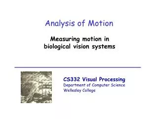
Analysis of Motion. Computing the velocity field. Measuring image motion. “aperture problem”. “local” motion detectors only measure component of motion perpendicular to moving edge. velocity field. 2D velocity field not determined uniquely from the changing image.

E N D
Analysis of Motion Computing the velocity field
Measuring image motion “aperture problem” “local” motion detectors only measure component of motion perpendicular to moving edge velocity field 2D velocity field not determined uniquely from the changing image need additional constraint to compute a unique velocity field
Assume pure translation or constant velocity Vy • Error in initial motion measurements • Velocities not constant locally • Image features with small range of orientations Vx In practice…
Smoothness assumption: • Compute a velocity field that: • is consistent with local measurements of image motion (perpendicular components) • has the least amount of variation possible
When is the smoothest velocity field correct? When is it wrong? motion illusions
Measuring motion in one dimension I(x) Vx x • Vx = velocity in x direction • rightward movement: Vx > 0 • leftward movement: Vx < 0 speed: |Vx| • pixels/time step I/x + - + - I/t I/t I/x Vx = -
Measurement of motion components in 2-D (1) gradient of image intensity I = (I/x, I/y) (2) time derivative I/t (3) velocity along gradient: v movement in direction of gradient: v > 0 movement opposite direction of gradient: v < 0 +x +y true motion motion component I/t [(I/x)2 + (I/y)2]1/2 I/t |I| v = - = -
2-D velocities (Vx,Vy) consistent with v (Vx, Vy) (Vx, Vy) Vy v Vx All (Vx, Vy) such that the component of (Vx, Vy) in the direction of the gradient is v (ux, uy): unit vector in direction of gradient Use the dot product: (Vx, Vy) (ux, uy) = v Vxux + Vyuy = v
Time-out exercise Vy Vx
Details… I/x = 10 I/y = -10 I/t = -30 (Vx, Vy) ?? I/x = 10 I/y = 10 I/t = -30 • For each component: • ux • uy • v • Vxux + Vyuy = v solve for Vx, Vy
In practice… Previously… Vy Vxux + Vy uy = v New strategy: Find (Vx, Vy) that best fits all motion components together Vx Find (Vx, Vy) that minimizes: Σ(Vxux + Vy uy - v)2
Computing the smoothest velocity field (Vxi-1, Vyi-1) motion components: Vxiuxi + Vyi uyi= vi (Vxi, Vyi) (Vxi+1, Vyi+1) i-1 i i+1 change in velocity: (Vxi+1-Vxi, Vyi+1-Vyi) Find (Vxi, Vyi) that minimize: Σ(Vxiuxi + Vyiuyi - vi)2 + [(Vxi+1-Vxi)2 + (Vyi+1-Vyi)2]