Download
1 / 70
700 likes | 843 Vues
CS4413 Sorting Algorithms II (These materials are used in the classroom only). Bubble Sort. Named because the elements get “bounced around” (exchanged) until they fall into the correct order. Like a sequential search, bubble sorts begin at one end and compare elements down the line.

E N D
CS4413 Sorting Algorithms II (These materials are used in the classroom only)
Bubble Sort • Named because the elements get “bounced around” (exchanged) until they fall into the correct order. • Like a sequential search, bubble sorts begin at one end and compare elements down the line. • When no exchange is needed, the sort is completed.
Bubble Sort … • Algorithm BubbleSort (A[0, …, n -1]) • //input: an array A[0, …, n -1] of orderable elements • //output: array A[0, …, n – 1] sorted in ascending order • for i ← 0 to n - 2 do • for j ← 0 to n - 2 - i do • if A[j + 1] < A[j] swap A[j] and A[j + 1]
Bubble Sort … • Most frequently used sorting algorithm. • Algorithm: • for i=0 to n - 2 …. O(n) • for j=0 to n - 2 - i ….. O(n) • if A[i] and A[i+1] are out of order, swap them • (that’s the bubble) …. O(1) • Analysis • Bubblesort is O(n2) • Appropriate for small arrays. • Appropriate for nearly sorted arrays. • Comparison versus swaps ?
Bubble Sort … • Compares adjacent items and swaps them if they are out of order • 1st pass - largest item in place • 2nd pass - 2 largest items in place • 3rd pass - 3 largest items in place • N-1pass - N largest items in place • If no swaps are made during a pass, done
Bubble Sort Analysis • N-1 passes • Pass 1: N-1 compares + at most N-1 swaps (3 moves each) • Pass 2: N-2 compares + at most N-2 swaps (3 moves each) • Worst case • N(N-1)/2 compares + N(N-1)/2 swaps * 3 moves per swap = 2N(N-1) = 2N2 -2N = O(N2)
Bubble Sort … • Not a particularly good algorithm. • Compare adjacent items and exchange them if they are out of order. Repeat. The largest item will eventually “bubble” to the correct position. • Pass 1 Pass 2 • 29 10 14 37 13 10 14 29 13 37 • 10 29 14 37 13 10 14 29 13 37 • 10 14 29 37 13 10 14 13 29 37 • 10 14 29 37 13 • 10 14 29 13 37 • …
Bubble Sort – Average case • N – 1 repetitions (passes) of the inner for loop in the worst case. • We need to know how many comparisons are done in each of these possibilities. • If we stop after one pass, we have done N – 1 comparisons. • If we stop after two passes, we have done (N -1) + (N -2) comparisons.
Bubble Sort – Average case • Let C(i) denote how many comparisons are done on the first i passes of the for loop before we stop. • Hence, we have the average complexity • A(N) = 1/(N – 1) ∑ i=0N-2 C(i) (1) • C(i) =∑ j= 0n – 2 - i j • =∑ j=0N – 2 j - ∑ j=0ij • = (N -1)N/2 – (i-1)i/2 = (N2 – N – i2 + i)/2 (2)
Bubble Sort – Average case • Substitute equation (2) back into equation (1) • A(N) = 1/(N -1) ∑ i= 0N – 2(N2 – N – i2 + i)/2 • = O(N2) • See page 66 (Textbook) for the complete derivation.
Bubble Sort • Worst case: O(n2) • Average case: O(n2) • Best case (already sorted): O(n)
ShellSort • Insertion sort is slow. (why?) • Shellsort is a simple extension of insertion sort which gains speed by allowing exchanges of elements that are far apart. • The idea is to rearrange the file to give it the property that taking every hth element (starting anywhere) yields a sorted file.
Shellsort Algorithm Algorithm Shellsort (list, N) //list: the elements to be put into order //N: the number of elements in the list passes = └lg N┘ while (passes ≥ 1) do increment = 2passes – 1 for start = 1 to increment do InsertionSort( list, N, start, increment ) end for passes = passes – 1 end while
ShellSort … • The algorithm analysis is to first determine the number of times we call the InsertionSort function and the number of elements in the lists for those calls. • A complete analysis of the shell sort is very complex and hence not covered in most textbooks. • The worst case is O(N3/2). • Shellsort is unique in that its general algorithm stays the same, but the choices of its parameters can have a dramatic effect on its order.
Radix Sorting • Radix sort uses key values to do the sort without actually comparing them to each other. • Create a set of ‘buckets” and distribute the entries into the buckets based on their key values. • After collecting the values and repeating this process for successive parts of the key, we can create a sorted list. • A process similar to this was used to sort cards in some libraries manually in earlier days.
Radix Sorting … • Uses linked lists • Idea: Multiple passes of Bucket Sort • Trick: Iteratively sort by last index, next to last, etc. • Example ed ca xa cd xd bd pass1: a:{ca, xa} d:{ed, cd, xd, bd} ca xa ed cd xd bd pass 2: b{bd} c: {ca, cd} e: {ed} x:{xa, xd} bd ca cd ed xa xd • Complexity: O(N* number of passes) • number of passes = length of key
Radix Sorting … • Uses the idea of forming groups and then combining them. The sort treats each data item as a character string. • Original Collection: • ABC, XYZ, BWZ, AAC, RLT, JBX, RDT • Grouped by rightmost letter: • (ABC, AAC) (RLT, RDT) (JBX) (XYZ, BWZ) • Next: • (AAC) (ABC, JBX) (RDT) (RLT) (BWZ) (XYZ)
Radix Sorting … • Last: • AAC, ABC, BWZ, JBX, RDT, RLT, XYZ • Algorithm: • Nested for loop • Order of magnitude: O(n) • Why are we using other sorting algorithms more often? • Space efficiency.
Radix Sorting … • Algorithm RadixSort (list, N) • //list: the elements to be put into order • //N: the number of elements in the list • Shift = 1 • for loop = 1 to keySize do • for entry = 1 to N do • bucketNumber = (list[entry].key /shift) mod 10 • Append (bucket[bucketNumber], list[entry]) • end for entry • list = CombineBuckets( ) • shift = shift * 10 • end for loop
Merge Sort • Merge sort is the first of our recursive sort algorithm. • Based on the idea that merging two sorted lists can be done quickly. • It breaks the list in half as long as first is less than last. • When we get to a point where first and last are equal, we have a list of one element, which is inherently sorted.
Merge Sort • When we return from the two calls to MergeSort that have lists of size 1, we then call MergeLists to put those together to create a sorted list of size 2. • At the next level up, we will have two lists of size 2 that get merged into one sorted list of size 4. • This process continues until we get to the top call, which merges the two sorted halves of the list back into one sorted list.
Merge Sort • Divide and Conquer…recursive solution. • Divide the collection in half , sort each half, then merge. Requires the use of a temporary array • Original array: 8 1 4 32 • Split: 8 1 4 3 2 • Sort: 1 4 8 2 3 • Merge: 1 2 3 4 8
Merge Sort • Algorithm: • Mergesort the first half of the array • Mergesort the second half of the array • Merge the sorted halves • Average case: O(n * logn)
Merge Sort • Let A be array of integers of length n • define Sort (A) recursively via auxSort(A,0,N) where • Define array[] Sort(A,low, high) • if (low == high) return • Else • mid = (low+high)/2 • temp1 = sort(A,low,mid) • temp2 = sort(A,mid,high) • temp3 = merge(temp1,temp2)
Merge Sort • Int[] Merge(int[] temp1, int[] temp2) • int[] temp = new int[ temp1.length+temp2.length] • int i,j,k • repeat • if (temp1[i]<temp2[j]) temp[k++]=temp1[i++] • else temp[k++] = temp2[j++] • for all appropriate i, j. • Analysis of Merge: • time: O( temp1.length+temp2.length) • memory: O(temp1.length+temp2.length)
Analysis of Merge Sort • Time • Let N be number of elements • Number of levels is O(logN) • At each level, O(N) work • Total is O(N * logN) • This is best possible for sorting.
Analysis of Merge Sort • Space • At each level, O(N) temporary space • Space can be freed, but calls to new costly • Needs O(N) space • Bad - better to have an in place sort • Quick Sort is the sort of choice.
Quicksort • QuickSort - fastest algorithm • QuickSort(S) • 1. If size of S is 0 or 1, return S • 2. Pick element v in S (pivot) • 3. Construct L = all elements less than v and R = all elements greater than v. • 4. Return QuickSort(L), then v, then QuickSort(R) • Algorithm can be done in situ (in place). • On average runs in O(N logN), but can take O(N2) time • depends on choice of pivot.
Quicksort: Analysis • Worst Case: • T(N) = worst case sorting time • T(1) = 1 • if bad pivot, T(N) = T(N-1)+N • Via Telescope argument (expand and add) • T(N) = O(N2) • Average Case (text argument) • Assume equally likely subproblem sizes • Note: chance of picking ith is 1/N • T(N) average cost to sort
Quicksort: Analysis • T(left branch) = T(right branch) (average) so • T(N) = 2 * ( T(0) + T(1)….T(N-1) )/N + N, where N is cost of partitioning • Multiply by N: • N T(N) = 2(T(0)+…+T(N-1)) +N2 (*) • Subtract N-1 case of (*) • N T(N) - (N-1) T(N-1) = 2 T(N-1) +2N - 1 • Rearrange and drop -1 • NT(N) = (N+1)T(N-1) + 2N - 1 • Divide by N(N+1) • T(N) / (N+1) = T(N-1) + 2 / (N+1)
Quicksort: Analysis • Substitute N-1, N-2,... 3 for N • T(N-1)/N = T(N-2)/(N-1) + 2/N • … • T(2)/3 = T(1)/2 + 2/3 • Add • T(N)/(N+1) = T(1)/2 + 2(1/3 + 1/4 + ..+ 1/(N + 1) • = 2( 1 + 1/2 +…) - 5/2 since T(1) = 0 • = O(logN) • Hence T(N) = N logN • In literature, more accurate proof. • For better results, choose pivot as median of 3 random values.
Quicksort • Another recursive divide and conquer sorting solution. • Partitions the collection by establishing a pivot point. On one side of the pivot are the numbers that are greater than the pivot and the other side contains the numbers that are less than the pivot.
Quicksort Original array: 5 3 6 7 4 Establish 5 as the pivot 5 | 3 6 7 4 5 | 3 | 6 7 4 5 | 3 | 6 | 7 4 5 | 3 | 6 | 7 | 4 5 | 3 4 | 6 7 3 4 5 6 7 pivot inserted Algorithm: Select pivot and partition Quicksort(S1 region of A) Quicksort(S2 region of A)
Balanced trees: AVL trees • For every node, difference in height between left and right subtree is at most 1. • AVL property is maintained through rotations, each time the tree becomes unbalanced. • lg n≤h≤ 1.4404 lg (n + 2) - 1.3277 average: 1.01 lg n + 0.1 for large n
Balanced trees: AVL trees • Disadvantage: needs extra storage for maintaining node balance. • A similar idea: red-black trees (height of subtrees is allowed to differ by up to a factor of 2).
AVL tree rotations • Small examples: • 1, 2, 3 • 3, 2, 1 • 1, 3, 2 • 3, 1, 2 • Larger example: 4, 5, 7, 2, 1, 3, 6 • See figures 6.4, 6.5 for general cases of rotations;
Balance factor • Algorithm maintains balance factor for each node. For example:
Heapsort Definition: A heap is a binary tree with the following conditions: • it is essentially complete: • The key at each node is ≥ keys at its children.
Definition implies: • Given n, there exists a unique binary tree with n nodes that is essentially complete, with h= lg n • The root has the largest key. • The subtree rooted at any node of a heap is also a heap.
Heapsort Algorithm: • Build heap. • Remove root –exchange with last (rightmost) leaf. • Fix up heap (excluding last leaf). Repeat 2, 3 until heap contains just one node.
Heap construction • Insert elements in the order given breadth-first in a binary tree. • Starting with the last (rightmost) parental node, fix the heap rooted at it, if it does not satisfy the heap condition: • exchange it with its largest child. • fix the subtree rooted at it (now in the child’s position). Example: 2 3 6 7 5 9
Root deletion The root of a heap can be deleted and the heap fixed up as follows: • exchange the root with the last leaf. • compare the new root (formerly the leaf) with each of its children and, if one of them is larger than the root, exchange it with the larger of the two. • continue the comparison/exchange with the children of the new root until it reaches a level of the tree where it is larger than both its children.
1 2 3 4 5 6 9 5 3 1 4 2 Representation • Use an array to store breadth-first traversal of heap tree: • Example: • Left child of node j is at 2j • Right child of node j is at 2j+1 • Parent of node j is at j /2 • Parental nodes are represented in the first n /2 locations 9 5 3 1 4 2