Download
1 / 44
440 likes | 457 Vues
This study explores the use of approximation algorithms for NP-Complete problems, including SAT, 3-SAT, Vertex Cover, and Partition. The goal is to design new algorithms that can be applied in various business application areas.

E N D
Exploring Approximation Algorithms and Their Empirical Analysis for Selected NP-Complete Problems By Roger G. Doss Northcentral University Prescott Valley, Arizona April 2011
Exploring Approximation Algorithms – Chapter 1 • NP Completeness theory evolved from the discovery of Cook's theorem. • Cook stated that the Satisfiability problem (SAT) requires exponentially many steps to compute in the worst case. • Cook's theorem is also known as Satisfiability (SAT). • At the time, it wasn’t known if there were any such NP-Complete problems.
Exploring Approximation Algorithms – Chapter 1 • Cook stated: Given an expression of Boolean variables in conjunctive normal form (CNF), finding an assignment of 0 or 1 values such that the expression evaluates to a true answer requires that one try all possibilities in the worst case. • Intuitively, a generic Boolean expression such as the logical AND operation x1 ^ x2 has the following truth assignment: • x1 ^ x2 • 0 0 0 • 0 1 0 • 1 0 0 • 1 1 1
Exploring Approximation Algorithms – Chapter 1 • There are 2n possibilities, so for two variables we have 4 possible states. Furthermore, if only the first 3 states are tried, we can not conclude that there is a false answer even though all three states produce a false answer. All four possibilities must be tried, hence the worst case of O(2n). • Conjunctive normal form (CNF) is a set of clauses containing Boolean variables that are logically OR'd together wherein the clauses are logically AND together. For example: • (x1 V x2 V x3) ^ (x4 V x5 V x6) • Each clause can be thought of as a variable which is AND together, and hence the need to try all possibilities as in the intuitive example.
Exploring Approximation Algorithms – Chapter 1 • Researchers expanded the theory to include problems that can be transformed from SAT. The most direct problem is 3-SAT. • In 3-SAT, the clauses must contain exactly three Boolean variables. • 3-SAT can represent all formula of SAT but allows for more structure and can be better utilized in proofs. • The 2-SAT problem, that is, having clauses of just two variables, can not logically represent all the possible formulas of 3-SAT and therefore is not equivalent to SAT. It is not NP-Complete. • Additional problems are Vertex Cover and Partition.
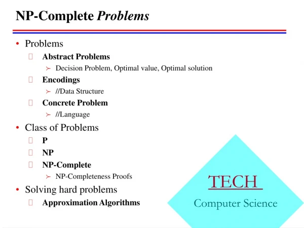
Exploring Approximation Algorithms – Chapter 1 • These three problems: 3-SAT, Vertex Cover, and Partition formed the basis of this study and are examples of NP-Complete problems. • NP-Complete problems appear in many studies, including math, computer science, graph theory, operations research, and scheduling theory. • Operations research and scheduling theory are directly related to scientific management and therefore business. • The problem is to design new Approximation Algorithms for these problems to facilitate business application areas such as Internet Search, Online Advertising, Resource Scheduling, and Expert System Design.
Exploring Approximation Algorithms – Chapter 2 • Literature Review • Provided information on background Computer Science theory. • Provided information on Theory of NP-Completeness. • Provided information on Approximation Algorithms. • Provided survey of related algorithms. • Provided examples of algorithm design techniques.
Exploring Approximation Algorithms – Chapter 2 • Types of Approximation Algorithms: • Greedy – always try to select the best possible case. • Divide and conquer – break the problem down to smaller tasks and solve. • Heuristics – use an observation or rule of thumb. • Genetic Algorithms – attempt to evolve a solution. • Meta approximations – utilize multiple approximations to solve a problem. • Random – utilize random variables in the design.
Exploring Approximation Algorithms – Chapter 2 • Approximations used in the study utilized: • Heuristics • Partition Approximation • Vertex Cover Approximation • Randomness • 3-SAT Approximation
Exploring Approximation Algorithms – Chapter 2 • Big-Oh notation refers to the order of an algorithm. • Algorithm performance is described as a function of input size n. • Polynomial time algorithms are the class P. • Nondeterministic Polynomial time algorithms are the class NP. • O(n), O(nlogn), O(logn) are examples of class P. • O(2n) is an example of class NP.
Exploring Approximation Algorithms – Chapter 2 • NP Completeness proofs: • Provide a polynomial time reduction from a known NP-Complete problem to a problem of unknown complexity. • The reduction maps the input of one problem to that of another. • Argue that if one problem is true the other is true, and vice versa (if and only if). • Implies the problem is at least as hard as the other. • Completeness means all problems that are NP-Complete can be reduced to each other.
Exploring Approximation Algorithms – Chapter 2 • Worst case scenario: • Order of algorithms is usually given in terms of the worst case. • For NP-Complete problems, the worst case is O(2n). • Want the average case as it is usually better than worst case. • Average case can be computed using empirical studies.
Exploring Approximation Algorithms – Chapter 2 • Note on performance: • An algorithm can have a good running time (<= O(N2)) in the worst case and still perform badly in practice as the details of the implementation are important along with the size of the input. • An algorithm can have a bad running time (O(2n)) in the worst case and not necessarily perform as badly in practice. In particular, the problem may have a good approximation which approaches the correct answer in a faster way.
Exploring Approximation Algorithms – Chapter 2 • Intractability: • There are two types of intractable problems. • These are non-solvable problems and solvable problems that are not computable optimally. • An example of a non-solvable problem is the halting problem. • Solvable problems that are not computable optimally are NP-Complete. • There are also problems that are hard, but not currently known to be NP-Complete such as factoring. • It is not known mathematically if P = NP. Are NP-Complete problems hard but currently no algorithm has been found, or that no algorithm can exist?
Exploring Approximation Algorithms – Chapter 2 • Approximations: • Mathematicians devised a way to deal with NP-Complete problems. • Instead of looking for an optimal solution, relax the problem to an acceptable solution. • Consider B an optimal solution for an NP-Complete problem. An algorithm necessarily has B = f(x) where x is an instance of the NP-Complete problem, and f(x) is a computation leading to the optimal solution B. • An approximation relaxes the restriction on f to be B <= f(x) <= k * B. • Where a desirable goal has k = 2. • Since B = f(x) is not possible.
Exploring Approximation Algorithms – Chapter 3 • The study conducted was an Applied Computer Science study. • Developed framework to study the approximations in the average case. • Implemented the optimal and approximation algorithms for three NP-Complete problems. • Developed 180 test cases with data generated randomly. • Compared the output of the optimal algorithm with the approximations for performance and accuracy. • Scripts where developed to run the experiment, capture data, and process in SPSS. • Utilized paired t-tests as we controlled for the variability of the input.
Exploring Approximation Algorithms – Chapter 3 • The optimal algorithm has the following design:
Exploring Approximation Algorithms – Chapter 3 • The optimal was used in the study inline with the literature. • It is sufficient to argue a performance increase and reasonable accuracy within a factor of 2 of the optimal. • It is not possible that an approximation produces a more accurate result than optimal. • The optimal was constructed for input <= 20 variables. • Implemented using multiple threads, employing techniques of randomized enumeration and early termination. • NP-Complete problems remain in NP regardless of the input size.
Exploring Approximation Algorithms – Chapter 3 • Randomized input: • The randomized input algorithms for 3-SAT, Vertex Cover, and Partition generate random instances of the respective problems. This is from statistics, where our samples are random. • For SAT, we generate a random number of variables, a random number of clauses and assign variables to clauses at random. • For VC, we generate a random number of vertexes and assign a random number of edges. • For Partition, we generate random number of tasks and task costs.
Exploring Approximation Algorithms – Chapter 3 • Partition • The Partition approximation had the following design: • Consider a pivot value, P, and a goal B = sum(tasks)/2 • If (P > B) => no solution is possible as P can not be subdivided. • If (P == B) => solution is {P}, {remainder of tasks} • Otherwise, P < B, therefore
Exploring Approximation Algorithms – Chapter 3 • order tasks from greatest to smallest value • let i be the index of the next task such that: • if ((P + task[i]) == B) => we are done, otherwise • (P + task[i]) < B, therefore • find next task i+1 such that: • if ((P + task[i] + task[i+1]) == B) => we are done, otherwise • (P + task[i] + task[i+1]) < B, therefore • find next task i+2 • And so on.
Exploring Approximation Algorithms – Chapter 3 • If we do not find a set of tasks that equal B, we repeat the process again using P as the starting point, but instead of combining it with task[i] as a start, we use task[i+1] as a start. • Then search again. • After trying n2 possibilities, we may select the one with the smallest difference if there was no combination that lead to the bound B. • NOTE: For very large data sets, we may try a single pass to avoid performing all n2 trials. • Approximation was 2 * OPT in the average case.
Exploring Approximation Algorithms – Chapter 3 • Numeric example: • 1 2 3 4 5 7 • Goal B is 22/2=11 • P = 7 (largest number < B) • try: 7 and select from 5 4 3 2 1 • next pick is 7 + 4 == 11 • NOTE: We do not pick 7 + 5 as this is > B • 7 + 4 yields a partition of {7,4} and {5,3,2,1} (both sides equal to B)
Exploring Approximation Algorithms – Chapter 3 • Vertex Cover: • A Vertex Cover is a set of vertexes such that every edge in the graph has an endpoint that is in the set. • The concept can be viewed as a graph representation of the most important members of a social network or the most relevant web pages in web search. • The approximation algorithm works by selecting the vertex with the highest degree (most edges connected to it). • Then adds this vertex to the Vertex Cover. • Then removes all edges associated with that vertex. • Then re-compute the vertex with the highest degree. • Repeats until a cover is reached.
Exploring Approximation Algorithms – Chapter 3 • At each iteration, it creates a new graph that is adapted based on the removal of the highest degree vertex and its adjacent edges. • Algorithm stops when a cover is made. • In the absolute worst case, the number of vertexes in the cover is equal to the number of vertexes in the graph. • In the average case, the approximation was 1.02 * OPT.
Exploring Approximation Algorithms – Chapter 3 • To visualize the approximation algorithm in operation, consider the following graph where the cover would be vertexes a and b:
Exploring Approximation Algorithms – Chapter 3 • 3-SAT • 3-SAT approximation works by considering 7 of the possible 8 states that can enable a 3 variable clause to be true. • The case that was eliminated was the case of all 0 values. • An assignment is selected by generating a pseudo-random number and taking the value modulo 7. • The number 7 is prime and therefore all numbers except 1 and 7 are relatively prime to it.
Exploring Approximation Algorithms – Chapter 3 • This produces a better distribution of values. • The approximation goes through a fixed number of iterations, where each trial is one of four separate paths in a random number generator. • Each path is run in a separate thread. • The algorithm can be configured based on number of threads and number of trials. • The approximation was 1 * OPT in the average case.
Exploring Approximation Algorithms – Chapter 4 Partition performance (opt vs. approx).
Exploring Approximation Algorithms – Chapter 4 Partition accuracy (opt vs. approx).
Exploring Approximation Algorithms – Chapter 4 Vertex Cover performance (opt vs. approx).
Exploring Approximation Algorithms – Chapter 4 Vertex Cover accuracy (opt vs. approx).
Exploring Approximation Algorithms – Chapter 4 3-SAT performance (opt vs. approx).
Exploring Approximation Algorithms – Chapter 4 3-SAT accuracy (opt vs. approx).
Exploring Approximation Algorithms – Chapter 4 • The first research question dealt with the performance of the proposed approximation algorithm for Partition Scheduling in comparison with the optimal algorithm. • The research findings showed that the null hypothesis can be rejected as there is significant difference in performance. The approximation is faster. • The second research question dealt with the accuracy of the proposed approximation for Partition Scheduling in comparison with the optimal. • The research findings showed that the null hypothesis can be rejected. The optimal here is more accurate; however, the approximation is within a factor of 2 * OPT.
Exploring Approximation Algorithms – Chapter 4 • The third research question dealt with the performance of the proposed approximation algorithm for Vertex Cover in comparison to the optimal. • The research findings showed that the null hypothesis can be rejected. The approximation is faster than the optimal. • The fourth research question dealt with the accuracy of the proposed approximation for Vertex Cover in comparison to the optimal. • The research findings showed that the null hypothesis can be rejected. The optimal is slightly more accurate than the approximation; however, the approximation is within a factor of 1.02 * OPT.
Exploring Approximation Algorithms – Chapter 4 • The fifth research question dealt with the performance of the proposed approximation for 3-SAT in comparison to the optimal. • The research findings showed that the null hypothesis can be rejected. The approximation is faster than the optimal. • The sixth research question dealt with the accuracy of the proposed approximation for 3-SAT in comparison to the optimal. • The research findings showed that the null hypothesis can be accepted. The approximation matched the accuracy of the optimal. The approximation was within a factor of 1 * OPT.
Exploring Approximation Algorithms – Chapter 4 • For 3-SAT, The statistic: ((NrYesOpt - NrYesApprox)/ NrTrials) * 100 was 0% as the percentage of correct results for 3-SAT approximation was 100%. • For Vertex Cover, the percentage of correct results was 138/180 * 100 = 76.7%. • For Partition, the percentage of correct results was 126/180 * 100 = 70%.
Exploring Approximation Algorithms – Chapter 4 • Algorithm running times: • average 3-SAT approx time 54.089 • average 3-SAT optimal time 14,204.950 • average Vertex Cover approx time 3827.578 • average Vertex Cover optimal time 128,554,437.684 • average Partition approx time 153.44 • average Partition optimal time 1,192,706.69
Exploring Approximation Algorithms – Chapter 4 • Running Time Accuracy (difference from opt) • Partition .00012865 = 153.44/1192706.69 2.0487 = (1.25-.41)/.41 • Vertex Cover .00002967 = 3827.58/1.29E8 .021 = (15.07-14.76)/14.76 • 3-SAT .00380783 = 54.09/14204.95 0 = (1-1)/1 * 100
Exploring Approximation Algorithms – Chapter 5 • The fact that certain problems are not computable is important in business as not all problems can have an optimal solution. • These problems are common in practice and are studied theoretically. • Another example is the Traveling Salesman problem where we wish to optimize a route for a salesman traveling from city to city. This problem is also NP-Complete.
Exploring Approximation Algorithms – Chapter 5 • This research developed a framework for testing Approximation Algorithms empirically against the optimal algorithm. • Provided new Approximation Algorithms for three selected NP-Complete problems. • Provided results regarding the performance and accuracy of those Approximations.
Exploring Approximation Algorithms – Chapter 5 • Future work: • Using the VC approximation to rank websites/web pages in a search engine. Additional logic may be required to assert the traffic of a given node. Offers clean, transparent way for ranking web pages unlike the hidden indicators used by the leading search engines. • We can develop Partition approximation into business application logic for scheduling resources. • We can develop 3-SAT approximation as a SAT solver for expert system design. • The algorithms can be made available for further study. • The framework can be used for developing other approximations for NP-Complete problems.
Exploring Approximation Algorithms – Chapter 5 • Thank You