Download
1 / 76
770 likes | 1.3k Vues
Contents. Overview What is Multiphysics? COMSOL’s Methodology for Multiphysics The fully coupled approach The sequential and segregated approaches An example of multiphysics couplings in COMSOL Concluding remarks. Fluid-structure interaction, FSI in a micro sensor. What is Multiphysics?.

E N D
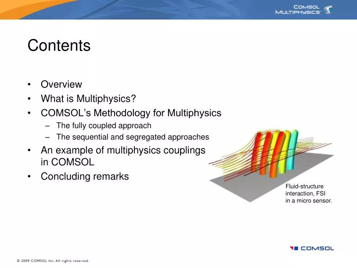
Contents • Overview • What is Multiphysics? • COMSOL’s Methodology for Multiphysics • The fully coupled approach • The sequential and segregated approaches • An example of multiphysics couplings in COMSOL • Concluding remarks Fluid-structure interaction, FSIin a micro sensor.
What is Multiphysics? • Multiphysics is the combination of several physics phenomena when describing a process • In modeling and simulations, these descriptions are based on the laws of physics • There is one precise way to present the laws of physics, and that is by means of differential equations* The description of a loudspeaker involves electromagnetic fields and forces, structural analysis, and acoustic pressure fields in the one model. * Feynman “Famous Lectures”
COMSOL’s Methodology for Modeling Multiphysics Phenomena • Development goals: • To create a software where scientists and engineers can formulate any system of partial differential equations (PDEs) based on the laws of physics • To formulate user interfaces, based on the above methods, for the most common areas in applied physics and engineering Microwave-thermal-structural multiphysics couplings in a waveguide circulator
COMSOL’s Methodology for Modeling Multiphysics Phenomena • Equation-based modeling • The modeling interface is based on an equation interpreter that formulates a finite element discretization, “on the fly”, for the fully coupled system • Predefined modeling interfaces for different fields of applied physics, including multiphysics couplings • Due to the underlying technology, properties, sources, sinks, and boundary conditions can be functions of the modeled variables and their partial derivatives • The full equations are also available in the user interface for further manipulation • Predefined interfaces can be combined with free PDE formulations directly in the user interface • Unlimited multiphysics formulations Electromagnetic fieldsand forces coupled to Newton’s law to compute the acceleration of a Maglev train
Solution of the coupled system COMSOL’s Methodology for Modeling Multiphysics PhenomenaExample: Fully Coupled Physics with Joule Heating and CFD • Definition in thegraphical user interface • Automatic assemblyusing equation interpretationand then discretization • Solution with direct or iterative solvers using a fullycoupled system utilizing a damped Newton method Fluid dynamicsand heat transfer Thermal analysis in solids Electromagenticfields Assembling of equations and discretization using FEM
COMSOL’s Methodology for Modeling Multiphysics PhenomenaExample: Fully Coupled Physics with Joule Heating and CFD • Temperature field defined in both solid and fluid domains • The fluid flow equations are only defined in the fluid domain • The static electric field is only defined in the solid domain Outlet Metal wire heatedusing an electric current Inlet
COMSOL’s Methodology for Modeling Multiphysics PhenomenaExample: Fully Coupled Physics with Joule Heating and CFD • Model Navigator: Select the combinations of physics • Draw Mode: Draw geometry or import it from a CAD file • Physics Mode: • Set material properties • Define multiphysics couplings and dependencies • Set boundary conditions • Mesh Mode: Select automatic or interactive meshing • Solve Mode: Solve the problem • Postprocessing Mode: Analyze the results
Available Modeling interfaces, called Application Modes. Select Add. Application Modes in the current model. Select ApplicationModes. Select Multiphysics
Note that u, v, w, p, V, and T are the dependent variables. Any function of these variables and their derivatives can be entered in the user interface. Select Add. Application Modes in the current model. Select ApplicationModes.
The Physics Settings and Material PropertiesThe Weakly Compressible Flow
Select the Weakly Compressible Navier-StokesApplication Mode from the Multiphysics menu… …or access it from the Model tree.
Select Physics and thenSubdomain Settings… …or access it from the Model tree.
For the air subdomain, Load air from the Material Library.
Properties are functions of T and p. This is the first multiphysics coupling!
Add patm (to be defined later) as thereference pressure. Stabilize densitywith respect to T (not necessary, but good to do).
Clear this check box to deactivate theflow equations in the hot-wire subdomain.
Select Physics, Boundary Settings for the flow problem… …or access it from the Model tree.
Select a fully developed Laminar inflow condition with an average value of U_inlet (to be defined later) at the Inlet.
Select a Pressure condition at the Outlet.
Set the Symmetry boundary.
Define patm, T_amb, and U_inlet in the Constants dialog box.
The Physics Settings and Material PropertiesThe Heat Transfer Settings
Select the Heat Transfer Application Mode.
Select Physics, Subdomain Settings for the Heat Transfer Application Mode. Load copper from the Material Library for the hot wire subdomain. Note that the heat source from Joule heating is automatically included. This is the second multiphysics coupling!
What does Q_emdc look like? It contains the components of the electric field, -Vx, -Vy, and –Vz… Answer: It is a predefined expression in the Equation System dialog box, which you do not need to open in this model, but which here shows the internally-used equation formulation. …which in turn defines the current density vector… …which then defines Q_emdc. Note that it is also possible to enter any function of V,Vx, Vy, and Vz directly in the edit fields in the subdomain or boundary settings (or any other variable and its derivatives).
Select the air subdomain and select Air as the Library material. Remove the heat source from Joule heating.
Select the Convection tab and Enable convective heat transfer. Enter u, v, and w (the flow velocity vector) to couple the Weakly Compressible Navier-Stokes Application Mode with Heat Transfer. This is the third multiphysics coupling!
The Physics Settings and Material PropertiesThe Conductive Media DC Settings
Switch to the Conductive Media DC Application Mode. Note the temperature dependent Electric conductivity, which defines the fourth multiphysics coupling.
Define Vm in the Constants menu in Options or from the Model tree.
This completes the physics settings for now. We can continue to the Mesh Mode. Select Ground for the base boundary of the hot wire. Select Electric insulation for the remaining boundaries.
Automatic meshing with tetrahedral elements. Quadrilateral and prism elements are also available as well as manual settings and adaptive meshing.
Just click the Solve button. The default solver is an iterative solver, which in the linear steps also uses an iterative procedure. A geometric multigridpreconditioner is used by default.
The slice plot shows temperature. The arrows show the velocity field. Note the expansion due to the temperature increase. The boundary plot on the hot wire shows the electric potential. The solution takes 12 minutes on a Toshiba Tecra laptop. It requires about 600 Mb of RAM including a 300 Mb footprint.
Concluding Remarks Regarding this Model • The model can be expanded in order to include buoyancy • It has negligible effect in this case but the CPU time does not increase • The model can be solved in the time domain. • This would then give the magnitude of the current flowing through the hot wire as a function of time and temperature • The model can be easily expanded to include a structural analysis • The thermal load is included as a volume load • The forces from the fluid are introduced as surface loads, so called fluid-structure interactions (FSI) • If large deformations occur, the displacements can be used in an ALE frame • The structural deformation affects the fluid flow path
Solution of the coupled system Solution of the Structural Analysis COMSOL’s Methodology for Modeling Multiphysics PhenomenaExample: Fully Coupled Physics with Joule Heating and CFD with weakly coupled FSI using a segregated approach Fluid dynamicsand heat transfer Thermal analysis in solids Electromagenticfields Structural Analysis,thermal expansion Assembling of equations and discretization using FEM This step is defined in the solver manager in the user interface, and does not require file transfers nor scripts. The segregationcan also be used for bidirectionalcoupling in order to save memory. T u,v,w
How difficult is it to add the Structural Analysis? Not difficult at all, it takes a few minutes…