Download
1 / 18
180 likes | 286 Vues
Variance. Fall 2003, Math 115B. Basic Idea. Tables of values and graphs of the p.m.f. ’s of the finite random variables, X and Y, are given in the sheet computations of the file v ariance example.xls .

E N D
Variance Fall 2003, Math 115B
Basic Idea • Tables of values and graphs of the p.m.f.’s of the finite random variables, X and Y, are given in the sheet computations of the file variance example.xls. • Let X be the random variable that gives the value of the die when a 10-sided die is rolled once. The sides of the die are labeled 1 through 5. • Let Y be the random variable that gives the average of the 2 sides of 10-sided die when it is rolled twice. The sides of the die are labeled 1 through 5.
Basic Idea (continued) • The mean of a distribution is a measure of center. • Although the means are the same, the concentration of the observations for each random variable is quite different. • The mean of the random variable does not accurately reflect where the probabilities lie • We need a parameter that measures the spread or dispersion of the possible values. • What is a parameter?
Computing Variance • Compute x - µX for all possible values of X. • What does this difference represent? • What happens when we sum all of these differences up? • Compute the sum of the squares of the deviations of the possible values from the mean. • Does not take into account the relative likelihood of the possible values of X. • Can weight each term with the probability of getting the value X.
Variance of a Finite Random Variable • We can now calculate (x - µX)2 * fX(x) • Each value of the p.m.f weights each term with the probability of obtaining the value x. • This weighted sum is called the variance of X, where X is a finite random variable • Denoted by V(X) • V(X) = Σ (x - µX)2 * fX(x), for all possible values of x • What does the variance tell us?
Standard Deviation • V(X) is one measure of dispersion. • The square root of V(X) is the preferred measure of dispersion. • Denoted by σX – called the standard deviation • Measured in the same units as X and µX • Interpreted as “typical amount” by which a value of X will differ from µX • σX ≥ 0
Example • The p.m.f of X, the number of Americans in a sample of size 4 that have at least 1 credit card is given to the right: • Find V(X) and σX
Special Case • What happens if X is a binomial random variable? • Then, V(X) = np(1-p) • Recall what n and p are • What does σX equal ? • Let X be the number of Americans with credit cards that pay off the full monthly balance • Take a sample size of 3 • The probability of success is 0.59 • Find V(X) and σX
Continuous Random Variable • Recall that the expected value, E(X), for a continuous r.v. is similar to the case for a finite r.v. • What are these formulas? • The same similarity occurs for the formulas for the variance • If X is a continuous random variable, what is V(X) and σX?
Example • Let X be the amount of time in minutes between arrivals/departures of planes at the Phoenix Sky Harbor airport • We know that α = 1.2 • What is fX(x)? • Set up, but do not evaluate, an integral that corresponds to • E(X) • V(X) • What happens when you integrate?
Example #2 • Let X be a continuous random variable with a uniform distribution over the interval [0,700] • What is fX(x)? • What is µX? • Using the above information, find • V(X) • σX
Samples • When the distribution of a random variable X is unknown, the pmf or pdf can be approximated by the histogram of a random sample for X and the mean of X can be estimated by the sample mean • How did we denote the sample mean? • Likewise for the variance of X • How do we denote the sample variance? • How do we denote the sample standard deviation?
Examples • A random sample for Y is given by 8,8,13,9,10,7,12,11,12,13 • Find s and s2 • A random sample for X, the number of Americans in a sample size 4 that have at least 1 credit card, is given by 2, 3, 4, 4, 3 • Find s and s2
Summary Chart • Taken directly from the course files, we have the following summary:
Sample Mean as a R.V. • We have a statistic, , that is being used to estimate the expected value • This statistic varies from sample to sample • I.e., it takes on different values • This statistic is a new random variable • We know the expected value of this random variable – what is it? • The variance and standard deviation of the sample mean are denoted by
Focus on the Project • Have continuous random variables V and R. • What do they represent? • We can now calculate the sample standard deviations of these random variables • Since we have no way of knowing the actual standard deviations of these random variables (why?), we will assume that the sample standard deviations are the same as the standard deviations • Let M be the continuous random variable that gives the sample mean for a set of 6 observations of R. • Then, E(M) = E(R) and
Standardization • Since we have two parameters, standard deviation and mean, we would like to know if knowing these two will characterize the distribution of a random variable, X. • If so, we could use these to determine probabilities • It turns out that we cannot • We can have two different r.v’s, X and Y • Have completely different shapes and different probabilities • They can have the same mean and standard deviation
Standardization • Can simplify computations by transforming a random variable • One of the most common is standardization • The standardization of X is given by • It can be shown that E(S) = 0 and σS = 1 • What does this mean? • This idea of standardization will continue throughout the rest of this project