Download
1 / 57
570 likes | 576 Vues
Making and Breaking Security Protocols with Heuristic Optimisation. John A Clark Dept. of Computer Science University of York, UK jac@cs.york.ac.uk IBM Hursley 13.02.2001. Overview. Introduction to heuristic optimisation techniques Part I: making security protocols

E N D
Making and Breaking Security Protocols with Heuristic Optimisation John A ClarkDept. of Computer Science University of York, UKjac@cs.york.ac.uk IBM Hursley 13.02.2001
Overview • Introduction to heuristic optimisation techniques • Part I: making security protocols • Part II: breaking protocols based on NP-hardness
x0 x1 x2 x3 Local Optimisation - Hill Climbing z(x) Really want toobtain xopt Neighbourhood of a point x might be N(x)={x+1,x-1}Hill-climb goes x0 x1 x2 since f(x0)<f(x1)<f(x2) > f(x3) and gets stuck at x2 (local optimum) xopt
x0 x1 x2 x4 x5 x6 x7 x8 x9 x10 x11 x12 x13 Simulated Annealing Allows non-improving moves so that it is possible to go down z(x) in order to rise again to reach globaloptimum x In practice neighbourhood may be very large and trial neighbour is chosen randomly. Possible to accept worsening move when improving ones exist.
Simulated Annealing • Improving moves always accepted • Non-improvingmoves may be accepted probabilistically and in a manner depending on the temperature parameter T. Loosely • the worse the move the lesslikely it is to be accepted • a worsening move is less likely to be accepted the cooler the temperature • The temperature T starts high and is gradually cooled as the search progresses. • Initially virtually anything is accepted, at the end only improving moves are allowed (and the search effectively reduces to hill-climbing)
Simulated Annealing • Current candidate x. Minimisation formulation. At each temperature consider 400 moves Always accept improving moves Temperature cycle Accept worsening moves probabilistically. Gets harder to do this the worse the move. Gets harder as Temp decreases.
Simulated Annealing Do 400 trial moves Do 400 trial moves Do 400 trial moves Do 400 trial moves Do 400 trial moves Do 400 trial moves
Genetic Algorithms • Based on evolution: survival of the fittest. • Encode solution to optimisation problem as a gene string. • Carry out the following (simple GA approach): • take a group of solutions • assess their fitness. • choose a new population with fitter individuals having more chance of selection. • ‘mate’ pairs to produce offspring. • allow individuals to mutate. • return to first step with offspring as new group. • Eventually the strings will converge to a solution.
Genetic Algorithms: Simple Example • The problem is: • maximise the function g(x)=x over the integers 0..15 • We shall now show how genetic algorithms might find this solution. • Let’s choose the obvious binary encoding of the integer solution space: • x=0 has encoding 0000 • x=5 has encoding 0101 • x=15 has encoding 1111 • Choose the obvious fitness function, fitness(x)=g(x)=x
a 0 0 1 1 3 b 0 1 0 0 4 a a 0 0 0 1 0 1 1 0 4 3 c 0 1 0 0 4 b b 0 0 1 0 0 1 0 1 3 4 d 0 0 1 1 3 c c 0 0 1 0 1 0 1 0 4 3 d d 0 0 0 0 1 1 1 0 3 2 14 Randomly choose pairs to mate, e.g. (a,b) and (c,d) with random cross-over points and swap right parts of genes 14 12 Randomly select 4 of these solutions according to fitness, e.g. b, a, a, c Randomly generate initial population a 0 0 0 0 0 a 0 0 0 0 0 b 0 1 1 1 7 Also allow bits to ‘flip’ occasionally, e.g. first bit of d. This allows a 1 to appear in the first column Now have radically fitter population, so continue to cycle. b 0 1 1 1 7 c 0 1 0 1 5 c 0 1 0 1 5 d 1 0 1 0 10 d 0 0 1 0 2 22 14 Genetic Algorithms: Simple Example
General Iteration • We now have our new generation, which is subject to selection, mating and mutation again......until some convergence criterion is met. • In practice it’s a bit more sophisticated but the preceding slide gives the gist. • Genetic algorithms have been found to be very versatile. One of the most important heuristic techniques of the past 30 years.
Security Protocols • Examples: • Secure session key exchange • “I am alive” protocols. • Various electronic transaction protocols. • Problems • Rather hard to get right • “We cannot even get three-line programs right” • Probably the highest profile area of academic security research. • Major impetus given to the area by Burrows Abadi and Needham’s belief logic “BAN logic”.
BAN Logic • Allows the assumptions and goals of a protocol to be stated abstractly in a belief logic. • Messages contain beliefs actually held by the sender. • Rules govern how receiver may legitimately update his belief state when he receives a message. • Protocols are series of messages. At the end of the protocol the belief states of the principals should contain the goals.
BAN Logic • Basic elements P,Q stand for arbitrary protocol principals K is a good key for communicating between P and Q Np is a well-typed ‘nonce’, a number to be used onlyonce in the current protocol run, e.g. a randomlygenerated number use as a challenge. Np is ‘fresh’ #, meaning that it really is a valid ‘nonce’
BAN Logic P once said X, i.e. has issued a message containing X at some point P believes X. The general idea is that principals shouldonly issue statements they actually believe. Thus, P mighthave believed that the number Na was fresh yesterdayand said so, but it would be wrong to conclude that hebelieves it now. If the message is recent (see later) then we might conclude he believes it. P has jurisdiction over X. This captures the notion that P is an authority about the statement X. If you believeP believes X and you trust him on the matter, then you should believe X too (see later)
BAN Logic - Assumptions and Goals A and S share common belief in the goodness of the key Kasand so they can use it to communicate. S also believes thatthe key Kab is a good session key for A and B. A has a number Na that he also believes is fresh and believes thatS is the authority on statements about the goodness of key Kab. The goal of the protocol is to get A to believe the key Kab is good for communication with B
If P sees X encrypted using key K and P believes that key K is shared securely only with principal Q then P should believe that Q once uttered or ‘once said’ X. BAN Logic –Message Meaning Rule
If P believes that Q once said X and P believes that X is ‘fresh’ then P should believe that Q currently believes X BAN Logic –Nonce Verification Rule This rule promotes ‘once saids’ to actual beliefs
If P believes that Q has jurisdiction over X and P believes Q believes X then P should believe X too BAN Logic – Jurisdiction Rule Jurisdiction captures the notion of being an authority. A typical use would be to give a key server authority over statements of belief about keys. If I believe that a key is good and you reckon I am an authority on such matters then you should believe the key is good too
4 3 2 1 0 Messages as Integer Sequences sender receiver Belief_1 Belief_2 22 19 8 12 0=22 mod 3 1=19 mod 3 3=8 mod 5 2=12 mod 5 P Q Say 3 principals P, Q and SP=0, Q=1,S=2 Message components are beliefs in thesender’s current belief state (and so if P has 5 beliefsintegers are interpreted modulo 5)
Search Strategy • We can now interpret sequences of integers as valid protocols. • Interpret each message in turn updating belief states after each message • This is the execution of the abstract protocol. • Every protocol achieves something! The issue is whether it is something we want! • We also have a move strategy for the search, e.g. just randomly change an integer element. • This can change the sender,receiver or specific belief of a message (and indeed subsequent ones)
Fitness Function • We need a fitness function to capture the attainment of goals. • Could simply count the number of goals attained at the end of the protocol • In practice this is awful. • A protocol that achieves a goal after 6 messages would be ‘good as’ ne that achieved a goal after 1 message. • Much better to reward the early attainment of goals in some way • Have investigated a variety of strategies.
Fitness Functions is given by One strategy (uniform credit) would be to make all the weightsthe same. Note that credit is cumulative. A goal achievedafter the first message is also achieved after the second andthird and so on.
Examples One of the assumptions made was that B would take S’sword n whether A |~Na
General Observations • Able to generate protocols whose abstract execution is a proof of their own correctness • Have done so for protocols requiring up to 9 messages to achieve the required goals. • Other methods for protocol synthesis is search via model checking. Exhaustive but limited to short protocols. • Can generalise notion of fitness function to include aspects other than correctness (e.g. amount of encryption).
Identification Problems • Notion of zero-knowledge introduced by Goldwasser and Micali (1985) • Indicate that you have a secret without revealing it • Early scheme by Shamir • Several schemes of late based on NP-complete problems • Permuted Kernel Problem (Shamir) • Syndrome Decoding (Stern) • Constrained Linear Equations (Stern) • Permuted Perceptron Problem(Pointcheval)
Given Find So That Pointcheval’s Perceptron Schemes • Interactive identification protocols based on NP-complete problem. • Perceptron Problem.
Given Find So That Has particular histogram H of positive values 1 3 5 .. .. .. Pointcheval’s Perceptron Schemes • Permuted Perceptron Problem (PPP). Make Problem harder by imposing extra constraint.
1 3 5 Example: Pointcheval’s Scheme • PP and PPP-example • Every PPP solution is a PP solution. Has particular histogram H of positive values
Generate random matrix A • Generate random secret S • Calculate AS • If any (AS)i <0 then negate ith row of A Generating Instances • Suggested method of generation: Significant structure in this problem; high correlation between majority values of matrix columns and secret corresponding secret bits
Image elements tend to be small 1 3 5 7… Instance Properties • Each matrix row/secret dot product is the sum of n Bernouilli (+1/-1) variables. • Initial image histogram has Binomial shape and is symmetric about 0 • After negation simply folds over to be positive -7–5-3-1 1 3 5 7…
Neighbourhood defined by single bit flips on current solution Cost function punishes any negative image components costNeg(y)=|-1|+|-3| =4 current solution Y PP Using Search: Pointcheval • Pointcheval couched the Perceptron Problem as a search problem.
Using Annealing: Pointcheval • PPP solution is also PP solution. • Based estimates of cracking PPP on ratio of PP solutions to PPP solutions. • Calculated sizes of matrix for which this should be most difficult • Gave rise to (m,n)=(m,m+16) • Recommended (m,n)=(101,117),(131,147),(151,167) • Gave estimates for number of years needed to solve PPP using annealing as PP solution means • Instances with matrices of size 200 ‘could usually be solved within a day’ • But no PPP problem instance greater than 71 was ever solved this way ‘despite months of computation’.
Perceptron Problem (PP) • Knudsen and Meier approach (loosely): • Carrying out sets of runs • Note where results obtained all agree • Fix those elements where there is complete agreement and carry out new set of runs and so on. • If repeated runs give same values for particular bits assumption is that those bits are actually set correctly • Used this sort of approach to solve instances of PP problem up to 180 times faster than Pointcheval for (151,167) problem but no upper bound given on sizes achievable.
Actual Secret Run 1 Run 2 Run 3 Run 4 Run 5 Run 6 All runs agree All agree (wrongly) Profiling Annealing • Approach is not without its problems. • Not all bits that have complete agreement are correct. 1 -1
Knudsen and Meier • Have used this method to attack PPP problem sizes (101,117) • Needs hefty enumeration stage (to search for wrong bits), allowed up to 264 search complexity • Used new cost function w1=30, w2=1 with histogram punishment cost(y)=w1costNeg(y)+w2costHist(y)
Analogy Time I: Encryption Plaintext P The Black Box Assumption – essentially considering encryption only as a mathematical function. In the public arena only really challenged in the 90’s when attacks based on physical implementation arrived Key • Fault Injection Attacks (Belcore, and others) Ciphertext C • Paul Kocher’s Timing Attacks • Simple Power Analysis • Differential Power Analysis The computational dynamics of the implementation can leak vast amounts of information
Analogy Time II: Annealing Problem P The Black Box Assumption – virtually every application of annealing simply throws the technique at problem and awaits the final output. Is this really the most efficient use of information? Let’s look inside the box….. Initialisation data Final Solution C
Analogy Time III: Internal Computational Dynamics Problem P, e.g. minimise cost(y,A,Hist) The algorithm carries out 100 000s of cost function evaluations which guide the search. Initialisation data Why did it take the path it did? Bear in mind the whole search process is public and so we can monitor it. Final Solution C
Analogy Time IV: Fault Injection Warped or Faulty Problem P’ Invariably people assume you need to solve the problem at hand. Reflected in ‘well-motivated’ or direct cost functions Initialisation data What happens if we inject a ‘fault’ into the process? Mutate the problem into a similar but different one. Can we make use of the solutions obtained to help solve original problem? Final Solution C’
PP Move Effects • What limits the ability of annealing to find a PP solution? • A move changes a single element of the current solution. • Want current negative image values to go positive • But changing a bit to cause negative values to go positive will often cause small positive values to go negative. 7 6 5 4 3 2 1 0 7 6 5 4 3 2 1 0
Problem Fault Injection • Can significantly improve results by punishing at positive value K • For example punish any value less than K=4 during the search • Drags the elements away from the boundary during search. • Also use square of differences |Wi-K|2 rather than simple deviation 7 6 5 4 3 2 1 0
Problem Fault Injection • Comparative results • Generally allows solution within a few runs of annealing for sizes (201,217) • Number of bits correct is generally worst when K=0. • Best value for K varies between sizes (but can do profiling to test what it is) • Has proved possible to solve for size (401,417) and higher. • Enormous increase in power for essentially change to one line of the program • Using powers of 2 rather than just modulus • Use of K factor • Morals… • Small changes may make a big difference. • The real issue is how the cost function and the search technique interact • The cost function need not be the most `natural’ direct expresion of the problem to be solved. • Cost functions are a means to an end. • This is a form of fault injection on the problem.
Profiling Annealing • But look again at the cost function templates • Different weights w1 and w2 will given different results yet the resulting cost functions seem plausibly well-motivated. • We can view different choices of weights as different viewpoints on the problem. • Now carry out runs using the different costs functions. • Very effective – using about 30 cost functions have managed to get agreement on about 25% of the key with less than 0.5 bits on average in error • Additional cost functions remove incorrect agreement (but may also reduce correct agreement).
Radical Viewpoint Analysis Problem P Problem P1 Problem P2 Problem Pn-1 Problem Pn Essentially create mutant problems and attempt to solve them. If the solutions agree on particular elements then they generally will do so for a reason, generally because they are correct. Can think of mutation as an attempt to blow the search away from actual original solution
Profiling Annealing: Timing • Simulated annealing can make progress, typically getting solutions with around 80% of the vector entries correct (but don’t know which 80%) • But this throws away a lot of information – better to monitor the search process as it cools down. • Based on notion of thermostatistical annealing. • Watch the elements of the secret vector as the search proceeds. • Record the temperature cycle at which the last change to an elements value occurs, i.e. +1 to –1 or vice versa • At the end of the search all elements are fixed. • Analysis shows that some elements will take some values early in the search and then never subsequently change. • They get ‘stuck’ early in the search. • The ones that get stuck early often do so for good reason – they are the correct values.