Download
1 / 89
890 likes | 1.04k Vues
Evolution of statistical models of non-conservative particle interactions. Irene M. Gamba Department of Mathematics and ICES The University of Texas at Austin. Kinetics and Statistical Methods for Complex Particle Systems Lisbon, July 2009. Collaborators: A. Bobylev, Karlstad University.

E N D
Evolution of statistical models of non-conservative particle interactions Irene M. Gamba Department of Mathematics and ICES The University of Texas at Austin Kinetics and Statistical Methods for Complex Particle Systems Lisbon, July 2009 Collaborators: A. Bobylev, Karlstad University. Ricardo Alonso, UT Austin-Rice University, Carlo Cercignani, Politecnico di Milano Vladislav Panferov, CSU, Northridge, CA, Cedric Villani, ENS Lyon, France. S. Harsha Tharkbushanam, ICES and PROS more recently J. Canizo, S. Mischler, C. Mouhot (Paris IV)
Overview • Introduction to classical kinetic equations for elastic and inelastic • interactions: • The Boltzmann equation for binary elastic and inelastic collisions • * Description of interactions, collisional frequency and potentials • * Energy dissipation & heat source mechanisms • * Self-similar models • Interactions of Maxwell type – The Fourier transform Boltzmann problem • * Initial value problem in the space ofcharacterictic functions (Fourier transformed probabilities) • * Connection to the Kac – N particle model • * Extensions of the Kac N-particle model to multi-particle interactions * construction of self-similar solutions and their asymptotic properties. • * characterizations of theirprobability density functions: Power tails • * Applications to agent interactions: information percolation and M-game multilinear model • * Explicit self similar solutions to a non-linear equation with a cooling background thermostat
Some issues of variable hard and soft potential interactions • Dissipative models for Variable hard potentials with heating sources: • All moments bounded • Stretched exponential high energy tails Spectral - Lagrange solvers for collisional problems • Deterministic solvers for Dissipative models - The space homogeneous problem • FFT application - Computations of Self-similar solutions • Space inhomogeneous problems • Time splitting algorithms • Simulations of boundary value – layers problems • Benchmark simulations
Statistical transport from interactive/collisional kinetic models • Rarefied ideal gases-elastic:classical conservativeBoltzmann Transport eq. • Energy dissipative phenomena: Gas of elastic or inelastic interacting systems in the presence of a thermostat with a fixed background temperature өb or Rapid granular flow dynamics: (inelastic hard sphere interactions): homogeneous cooling states, randomly heated states, shear flows, shockwaves past wedges, etc. • (Soft) condensed matter at nano scale: Bose-Einstein condensates models and charge transport in solids: current/voltage transport modeling semiconductor. • Emerging applications from stochastic dynamics for multi-linear Maxwell type interactions : Multiplicatively Interactive Stochastic Processes: • information percolation models, particle swarms in population dynamics, Simulations of granular flows from UT Austin and CalTech groups • Goals: • Understanding of analytical properties: large energy tails • Long time asymptotics and characterization of asymptotics states • A unified approach for Maxwell type interactions and generalizations. • Spectral-Lagrangian solvers for dissipative interactions
Part I • Introduction to classical kinetic equations for elastic and inelastic interactions: The Boltzmann equation for binary elastic and inelastic collisions * Description of interactions, collisional frequency and potentials * Energy dissipation & heat source mechanisms * Self-similar models
Part I The classical Elastic/Inelastic Boltzmann Transport Equation for hard spheres: ( L. Boltzmann 1880's), in strong form: For f (t; x; v) = f and f (t; x; v*) = f*describes the evolution of a probability distribution function (pdf) of finding a particle centered at x ϵRd, with velocity v ϵRd, at time t ϵR+ ,satisfying u = v-v* := relative velocity |u · η| dη := collision rate elastic ‘v v u · η = uη :=impact velocity η := impact direction (random in S+d-1) inelastic η v* ‘v* u · η= (v-v*) .η = - e ('v-'v*) ·η= -e'u .η u · η ┴= (v-v*) ·η┴ = ('v-'v*) · η┴ = 'u · η ┴ γ C = number of particle in the box a = diameter of the spheres d = space dimension θ e := restitution coefficient : 0 ≤ e ≤ 1 e = 1 elastic interaction , 0 < e < 1 inelatic interaction, ( e=0 ‘sticky’ particles)
:= mass density :=statistical correlation function (sort of mean field ansatz,i.e. independent of v) = for elastic interactions (e=1) i.e. enough intersitial space May be extended to multi-linear interactions (in some special cases to see later)
it is assumed that the restitution coefficient is only a function of the impact velocity e = e(|u·n|). The properties of the map z e(z) are v' = v+ (1+e) (u .η) η and v'* = v* + (1+e) (u . η) η 2 2 The notation for pre-collision perspective uses symbols 'v, 'v* : Then, for 'e = e(| 'u · n|) = 1/e, the pre-collisional velocities are clearly given by 'v = v+ (1+'e) ('u .η) η and 'v* = v* + (1+'e) ('u . η) η 2 2 In addition, the Jacobian of the transformation is then given by J(e(z)) = e(z) + zez(z) = θz(z) =( z e(z) )z However, for a ‘handy’ weak formulation we need to write the equation in a different set of coordinates involving σ := u'/|u| the unit direction of the specular (elastic) reflection of the postcollisional relative velocity, for d=3 σ γ θ
Goal:Write the BTE in ( (v +v*)/2 ; u) = (center of mass, relative velocity) coordinates. Let u = v – v* the relative velocity associated to an elastic interaction. Let P be the orthogonal plane to u. Spherical coordinates to represent the d-space spanned by {u; P} are {r; φ; ε1; ε2;…; εd-2}, where r = radial coordinates, φ = polar angle, and {ε1; ε2;…; εd-2},the n-2 azimuthal angular variables. σ then with , θ= scattering angle • 0 ≤ sin γ = b/a ≤ 1, with b = impact parameter, a =diameter of particle • Assume scattering effects are symmetric with respect to θ = 0→ 0 ≤ θ≤ π ↔ 0 ≤ γ≤ π/2 • The unit direction σis the specular reflection of u w.r.t. γ, that is |u|σ = u-2(u · η) η • Then write the BTE collisional integral with the σ-directiondηdv* → dσ dv* , η, σ in Sd-1 • using the identity So the exchange of coordinates can be performed. In addition, since then any function b(u · σ) defined on Sd-1satisfies |u| dσ = |Sd-2| sind-2 θ dθ, 1 ∫Sd-1 b(|u · σ|)dσ = |Sd-2|∫0b(z) (1-z2) (d-3)/2 dz |u| , z=cosθ
Interchange of velocities during a binary collision or interaction σ= uref/|u| is the unit vector in the direction of the relative velocity with respect to an elastic collision v' u' v' θ u' σ . v σ v . . u u . η η e γ γ 1-β β v* v'* v* v'* Inelastic collision Elastic collision 1- β+e =β Remark: θ≈0 grazing and θ ≈ πhead oncollisions or interactions
Weak (Maxwell) Formulation: center of mass/ (specular reflected) relative velocity Due to symmetries of the collisional integral one can obtain (after interchanging the variables of integration) Both Elastic/inelastic formulations: The inelasticity shows only in the exchange of velocities. Center of mass-relative velocity coordinates for Q(f; f): 1-β σ= uref/|u| is the unit vector in the direction of the relative velocity with respect to an elastic collision γ γ = 0 for Maxwell Type (or Maxwell Molecule) models γ = 1 for hard spheres models; 0< γ<1 for variable hardpotential models, -d < γ< 0 for variable soft potential models. β
Collisional kernel or transition probability of interactions is calculated using intramolecular potential laws: is the angular cross section satisfies In addition, we shall use the α-growth condition which is satisfied for angular cross section function for α > d-1(in 3-d is for α>2)
Weak Formulation & fundamental properties of the collisional integral and the equation: Conservation of moments & entropy inequality x-space homogeneous (or periodic boundary condition) problem: Due to symmetries of the collisional integral one can obtain (after interchanging the variables of integration) Invariant quantities (or observables) - These are statistical moments of the ‘pdf’
Time irreversibility is expressed in this inequality stability In addition: The Boltzmann Theorem:there are only N+2 collision invariants
→yields the compressible Euler eqs→Small perturbations of Mawellians yield CNS eqs.
Exact energy identity for a Maxwell type interaction models Then f(v,t) → δ0ast → ∞ to a singular concentrated measure (unless there is ‘source’) Current issues of interest regarding energy dissipation: Can one tell the shape or classify possible stationary states and their asymptotics, such as self-similarity? Non-Gaussian (or Maxwellian) statistics!
Reviewing inelastic properties INELASTIC Boltzmann collision term: No classical H-Theorem if e= constant < 1 However, it dissipates total energy for e=e(z) < 1 (by Jensen's inequality): • Inelasticity brings loss of micro reversibility • but keeps time irreversibility!!: That is, there are stationary states and, in some particular cases we can show stability to stationary and self-similar states (Multi-linear Maxwell molecule equations of collisional type and variable hard potentials for collisions with a background thermostat) • However: Existence of NESS: Non Equilibrium Statistical States (stable stationary states are non-Gaussian pdf’s)
A general formstatistical transport : The space-homogenous BTE with external heating sources Important examples from mathematical physics and social sciences: The term models external heating sources: • background thermostat (linear collisions), • thermal bath (diffusion) • shear flow (friction), • dynamically scaled long time limits (self-similar solutions). ‘v v η v* ‘v* u’= (1-β) u + β |u| σ , with σthe direction of elastic post-collisional relativevelocity Inelastic Collision
The collision frequency is given by Qualitative issues on elastic: Bobylev,78-84, and inelastic: Bobylev, Carrillo I.G, JSP2000, Bobylev, Cercignani 03-04,with Toscani 03, with I.M.G. JSP’06, arXiv.org’06, CMP’09 Classical work of Boltzmann, Carleman, Arkeryd, Shinbrot,Kaniel, Illner,Cercignani, Desvilletes, Wennberg, Di-Perna, Lions, Bobylev, Villani, (for inelastic as well),Panferov, I.M.G,Alonso (spanning from 1888 to 2009) Qualitative issues on variable hard spheres, elastic and inelastic: I.G., V.Panferov and C.Villani, CMP'04, Bobylev, I.G., V.Panferov JSP'04, S.Mishler and C. Mohout, JSP'06, I.G.Panferov, Villani 06 -ARMA’09, R. Alonso and I.M. G., 07. (JMPA ‘08, and preprints 09)
Energy dissipation implies the appearance of Non-Equilibrium Stationary Statistical States
Part II • Interactions of Maxwell type – The Fourier transform Boltzmann problem * initial value problem in the space ofcharacterictic functions (Fourier transformed probabilities) * Connection to the Kac – N particle model * Extensions of the Kac N-particle model to multi-particle interactions * construction of self-similar solutions and their asymptotic properties. * characterizations of theirprobability density functions: Power tails * Applications to agent interactions: information percolation and M-game multilinear model
Motivation of maxwell type models for inelastic interactions (or Pseudo Maxwell molecule models) They can always be obtained by assuming that the relative speed |u| scales by a mean field quantity Example: Then, one obtains the Energy Identity So it is possible to obtain the (expected) polynomial time decay rate for the kinetic energy • In addition, we (Bobylev, Carrillo and I.M.G., JSP’00) were able to solve the initial value problem • by the method of Wild sums → Not quite, also the behavior of the kinetic solution is relevant as well Question:Is the kinetic decay rate what it matters for hydrodynamics?
Maxwell type of elastic or inelastic interactions (or Pseudo Maxwell molecule models) They can always be obtained by assuming that the relative speed |u| scales by a mean field quantity Example: Energy Identity • And for e constant we showed that: • large even moments of self-similar solutions become negative. (also in BCG JSP'00) • Existence of solution with power like velocity tails for a set of 0 < e < 1 and corresponding self-similar asymptotics and decay estimates.(Ernst-Brito JSP'02; Bobylev-Cercignani JSP'02; with Toscani; JSP'03) • for any 0 < e < 1: NOT all even moments can be bounded for initial data in L1k(Rd), for all e, (Bobylev,I.M.G.JSP'06 ) • Generalization to multi-linear energy conservative or dissipative collisional forms in Maxwell type model formulation with applications to kinetic mixtures with sources, social dynamical interactions, and more (Bobylev,Cercignani, I.M.G. '06)
Back to molecular models of Maxwell type (as originally studied) so is also a probability distribution function in v. Then: work in the space of “characteristic functions” associated to Probabilities: “positive probability measures in v-space are continuous bounded functions in Fourier transformedk-space” The Fourier transformed problem: Γ Bobylev operator characterized by One may think of this model as the generalization original Kac (’59) probabilistic interpretation of rules of dynamics on each time step Δt=2/M of M particles associated to system of vectors randomly interchanging velocities pairwise while preserving momentum and local energy, independently of their relative velocities. Bobylev, ’75-80, for the elastic, energy conservative case. Drawing from Kac’s models and Mc Kean work in the 60’s Carlen, Carvalho, Gabetta, Toscani, 80-90’s For inelastic interactions: Bobylev,Carrillo, I.M.G. 00 Bobylev, Cercignani,Toscani, 03, Bobylev, Cercignani, I.M.G’06 and 08, for general non-conservative problem
Recall fromFourier transform: nthmoments of f(., v) are nth derivatives of φ(.,k)|k=0 Θ And, for isotropic (x = |k|2/2 ) or self similar solutions (x = |k|2/2 eμt, μ is the energy dissipation rate, that is: Θt = - μΘ ),by performing the operations with , then, the Fourier transformed collisional operator is written Kd accounts for the integrability of the functionb(1-2s)(s-s2)(N-3)/2 For isotropic solutions the equation becomes (after rescaling in time the dimensional constant) φt + φ = Γ(φ , φ ) ; φ(t,0)=1, φ(0,k)=F (f0)(k), Θ(t)= - φ’(0) In this case, using the linearization of Γ(φ , φ ) about the stationary state φ=1, we can inferred the energy rate of change by looking at λ1 defined by kinetic energy is dissipated < 1 λ1:=∫10 (aβ(s) + bβ(s)) G(s) ds= 1kinetic energy is conserved > 1 kinetic energy is generated
Examples Existence, asymptotic behavior - self-similar solutions and power like tails: From a unified point of energy dissipative Maxwell type models: λ1energy dissipation rate(Bobylev, I.M.G.JSP’06, Bobylev,Cercignani,I.G. arXiv.org’06- CMP’08)
Existence: Wild's sum in the Fourier representation. The existence theorems for the classical elastic case ( β=e = 1) of Maxwell type of interactions were proved by Morgenstern,Wild 1950s, Bobylev 70s using the Fourier transform • rescale time t →τ and solve the initial value problem Γ Γ 1-β/2 β/2 β/2 by a power series expansion in time where the phase-space dependence is in the coefficients Wild's sum in the Fourier representation. Γ Note that if the initial coefficient |φ0|≤1, then |Фn|≤1 for any n≥ 0. the series converges uniformly for τϵ[0; 1).
Problem for (elastic) inelastic interaction (B-C-G, JSP’00) near a Dirac delta Spherical harmonic expansions For compact operators invariant under rotations
Problem for (elastic) inelastic interaction (B-C-G, JSP’00) such that Thus, as t →∞, it recovers conservation of energy Remark: Variable restitution coefficient: there are no self-similar solutions, but for small temperature or restitution coefficient uniformly close to 1, the homogeneous solution is close to the Maxwellian distribution as described before.
Remarks: -- Power like tails for econstant and self-similar asymptotics. (Ernst-Brito, Bobylev-Cercignani- JSP'02, with Toscani-JSP'03, Bobylev I.M.G, JSP’06) -- Generalization to global dissipative Kac-type models with multi linear interactions by Spectral Characteristic methods(Bobylev-Cercignani-I.M.G arXiv.org’06, 08,CMP’09)
Generalization of Maxwell to multi-linear interacting models • Motivation: Lays on the observation that quite different equations for probability dynamics leads to the same class of equations in the evolution equation for the Fourier (Laplace) representation for their characteristic (generating) functions. • Examples: • Kac caricature models for elastic particles • elastic or inelastic homogenous Boltzmann equation of Maxwell type interactions in • higher dimensions • models for slow down processes: background cooling (soft condensed matter phenomena) • statistical evolution in social dynamics by binary interactions • We present a canonical probabilistic model equivalent to generalized Maxwell molecule models: Ideas follow from the ‘same line of thought’ where only games with two players • were considered in MISP (or random interactive processes) ben-Avraham, Ben-Naim, Lindenberg & Rosas '03; Pareschi & Toscani '05-06, and Fujihara, Ohtsuki, & Yamamoto '06:
More generally (Bobylev, Cercignani and IMG, arXiv.org’06, 09, CMP’09) Connection between the kinetic Boltzmann equations and Kac probabilistic interpretation of statistical mechanics Consider a spatially homogeneous d-dimensional ( d ≥ 2) rarefied gas of particles having a unit mass. Let f(v, t), where v ∈ Rdand t ∈ R+, be a one-point pdf with the usual normalization Assumption: I - collision frequency is independent of velocities of interacting particles (Maxwell-type) II - the total scattering cross section is finite. Hence, one can choose such units of time such that the corresponding classical Boltzmann eqs. reads with Q+(f) is the gain term of the collision integral and Q+ transforms fto another probability density
The same stochastic model admits other possible generalizations. For example we can also include multiple interactions and interactions with a background (thermostat). This type of model will formally correspond to a version of the kinetic equation for some Q+(f). where Q(j)+ , j = 1, . . . ,M, are j-linear positive operators describing interactions of j ≥ 1 particles, and αj ≥ 0 are relative probabilities of such interactions, where • What properties of Q(j)+ are needed to make them consistent with the Maxwell-type interactions? • Temporal evolution of the system is invariant under scaling transformations of the phase space: • if St is the evolution operator for the given N-particle system such that • St{v1(0), . . . , vM(0)} = {v1(t), . . . , vM(t)} , t ≥ 0 , then St{λv1(0), . . . , λvM(0)} = {λv1(t), . . . , λvM(t)} for any constant λ> 0 which leads to the property Q+(j) (Aλ f) = AλQ+(j) (f), Aλf(v) = λd f(λv) , λ > 0, (j = 1, 2, .,M) Note that the transformation Aλ is consistent with the normalization of f with respect to v.
Property: Temporal evolution of the system is invariant under scaling transformations of the phase space: Makes the use of the Fourier Transform a natural tool so the evolution eq. is transformed is also invariant under scaling transformations k → λk, k ∈ Rd If solutions are isotropic then -∞ -∞ where Qj(a1, . . . , aj) can be an generalized functions of j-non-negative variables. • All these considerations remain valid for d = 1, the only two differences are: • The evolving Boltzmann Eq should be considered as the one-dimensional Kac master equation, • and one uses the Laplace transform • ( andconnects to the lecture of R. Pego) • 2. We discussed a one dimensional multi-particle stochastic model with non-negative phase • variables v in R+,
The structure of this equation follows from the well-known probabilistic interpretation by M. Kac:Consider stochastic dynamics of N particles with phase coordinates (velocities) VN=vi(t) ∈ Ωd, i = 1..N , with Ω= R or R+ A simplified Kac rules of binary dynamics is:on each time-step t = 2/N , choose randomly a pair of integers 1 ≤ i < l ≤ N and perform a transformation (vi, vl) →(v′i , v′l) which corresponds to an interaction of two particles with ‘pre-collisional’ velocities vi and vl. Then introduce N-particle distribution function F(VN, t) and consider a weak form of the Kac Master equation (we have assumed thatV’ Nj= V’N j ( VNj , UN j · σ) for pairs j=i,l with σ in a compact set) dσ ΩdN 2 ΩdN x Sd-1 Introducing a one-particle distribution function (by setting v1 = v) and the hierarchy reduction for B= -∞ or B=0 B B B The assumed rules lead (formally, under additional assumptions) to molecular chaos, that is The corresponding “weak formulation” forf(v,t) for any test function φ(v) where the RHS has a bilinear structure from evaluating f(vi’,t) f(vl’, t) M. Kac showed yields the the Boltzmann equation of Maxwell type in weak form (as in E. Carlen lecture) (or Kac’s walk on the sphere)
Rigorous results (Bobylev, Cercignani, I.M.G.;.arXig.org ’06, ’09,- CMP’09) Existence, stability,uniqueness, Θ with 0 < p < 1 infinity energy, or p ≥ 1 finite energy
(for initial data with finite energy) Relates to the work of Toscani, Gabetta,Wennberg, Villani,Carlen, Carvallo,…..
- I Boltzmann Spectrum
(Bobylev, Cercignani, I.M.G.;.arXig.org ’06, ’09,- CMP’09) Stability estimate for a weighted pointwise distance for finite or infinite initial energy These estimates are a consequence of the L-Lipschitz condition associated to Γ: they generalized Bobylev, Cercignani and Toscani,JSP’03 and later interpeted as “contractive distances” (as originally by Toscani, Gabetta, Wennberg, ’96) These estimates imply, jointly with the property of the invariance under dilations for Γ, selfsimilar asymptotics and the existence of non-trivial dynamically stable laws.
Existence of Self-Similar Solutions with initial conditions REMARK: The transformation , forp > 0 transforms the study of the initial value problem touo(x) = 1+x and ||uo|| ≤1 so it is enough to study the casep=1
In addition, the corresponding Fourier Transform of the self-similar pdf admits an integral representation by distributionsMp(|v|)with kernels Rp(τ) , for p = μ−1(μ∗). They are given by: Similarly, by means of Laplace transform inversion, for v ≥0 and 0 < p ≤ 1 with These representations explain the connection of self-similar solutions with stable distributions