An Introduction to R

1. An Introduction to R 指導教授：陳光琦  報告者：朱育正

2. An Introduction to R • The R environment • R and statistics

3. The R Environment • R 是一組資料操作，計算和圖形顯示工具的整合包。相對其他同類軟體，它的特色在於： 1.有效的資料處理和保存機制， 2.擁有一整套陣列和矩陣的操作運算符， 3.一系列連貫而又完整的資料分析中間工具

4. The R Environment 4.圖形工具可以對資料直接進行分析和顯示，可用於多種圖形設備， 5.一種相當完善，簡潔和高效的程式設計語言 (也就是 `S')。它包括條件語句，迴圈語句，用戶定義的遞迴函數以及輸入輸出介面。（實際上，系統提供的大多數函數都是用 S 寫的）。

5. The R Environment • 和其他資料分析軟體的一樣，術語“環境”（environment）是用來描述一個充分設計、連貫性的系統，而不是一個非常專一並且難以擴充的工具群。 • R 是一個開發新的互動式資料分析方法的工具。它的開發週期短，而且有大量的擴展包（packages）可以使用。

6. R and Statistics • 我們對 R 環境的介紹沒有提到 統計，但是大多數人用 R 就是因為它的統計功能。不過，我們寧可把 R 當作一個內部實現了許多經典的時髦的統計技術的環境。部分的統計功能是整合在 R 環境的底層，但是大多數功能則以 包 的形式提供。大約有25個包和 R 同時發佈（被稱為“標準” 和“推薦”包），更多的包可以通過網上或其他地方的 CRAN 社區 (http://CRAN.R-project.org) 得到。關於包更多的細節將在後面的章節敍述 (see Packages)。

7. R and Statistics • 大多數經典的統計方法和最新的技術都可以在 R 中直接得到。終端用戶只是需要花點精力去找到一下就可以了。 • S (因此也包括 R) 和其他主要的統計系統在觀念上有著重要的差異。在 S 語言中，一次統計分析常常被分解成一系列步驟，並且所有的中間結果都被保存在對象（object）中。因此，儘管 SAS 和 SPSS 為回歸和判別分析提供了豐富的螢幕輸出內容，但 R 給出螢幕輸出卻很少。它將結果保存在一些合適的物件中以便於用 R 裏面的函數做進一步的分析。

8. What R Does and Does Not • is not a database, but connects to DBMSs • has no graphical user interfaces, but connects to Java, TclTk • language interpreter can be very slow, but allows to call own C/C++ code • no spreadsheet view of data, but connects to Excel/MsOffice • no professional / commercial support • data handling and storage: numeric, textual • matrix algebra • hash tables and regular expressions • high-level data analytic and statistical functions • classes (“OO”) • graphics • programming language: loops, branching, subroutines

9. Data Analysis and Presentation • The R distribution contains functionality for large number of statistical procedures. • linear and generalized linear models • nonlinear regression models • time series analysis • classical parametric and nonparametric tests • clustering • smoothing • R also has a large set of functions which provide a flexible graphical environment for creating various kinds of data presentations.

10. Application • 下面的會話讓你在操作中對 R 環境的一些特性有個簡單的瞭解。你對系統的許多特性開始時可能有點不熟悉和困惑，但這些迷惑會很快消失的。 • 登錄，啟動你的桌面系統。 • $ R • 以適當的方式啟動 R1。 R 程式開始，並且有一段引導語。 • (在 R 裏面，左邊的提示符將不會被顯示防止混淆。) • help.start() • 啟動 HTML 形式的線上幫助(使用你的電腦裏面可用的流覽器)。你可以用滑鼠點擊上面的鏈結。 最小化幫助視窗，進入下一部分。

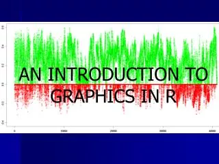
11. Application • x <- rnorm(50) • y <- rnorm(x) • 產生兩個偽正態亂數向量 x 和 y。 • plot(x, y) • 畫二維散點圖。一個圖形視窗會自動出現。

12. (cont’d) • ls() • 查看當前工作空間裏面的 R 物件。 • rm(x, y) • 去掉不再需要的物件。(清空)。 • x <- 1:20 • 等價於 x = (1, 2, ..., 20)。 • w <- 1 + sqrt(x)/2 • 標準差的`權重'向量。 • dummy <- data.frame(x=x, y= x + rnorm(x)*w) • dummy • 創建一個由x 和 y構成的雙列資料框，查看它們。

13. (cont’d) • fm <- lm(y ~ x, data=dummy) • summary(fm) • 擬合 y 對 x 的簡單線性回歸，查看分析結果。 • fm1 <- lm(y ~ x, data=dummy, weight=1/w^2) • summary(fm1) • 現在我們已經知道標準差，做一個加權回歸。 • attach(dummy) • 讓資料框中的列項可以像一般的變數那樣使用。 • lrf <- lowess(x, y) • 做一個非參局部回歸。 • plot(x, y) • 標準散點圖。

14. (cont’d) • lines(x, lrf$y) • 增加局部回歸曲線。 • abline(0, 1, lty=3) • 真正的回歸曲線：(截距 0，斜率 1)。 • abline(coef(fm)) • 無權重回歸曲線。 • abline(coef(fm1), col = "red") • 加權回歸曲線。

15. (cont’d) • detach() • 將資料框從搜索路徑中去除。 • plot(fitted(fm), resid(fm), •      xlab="Fitted values", •      ylab="Residuals", •      main="Residuals vs Fitted") • 一個檢驗異方差性（heteroscedasticity）的標準回歸診斷圖。你可以看見嗎？ • qqnorm(resid(fm), main="Residuals Rankit Plot") • 用正態分值圖檢驗資料的偏度（skewness），峰度（kurtosis）和異常值（outlier）。（這裏沒有多大的用途，只是演示一下而已。） • rm(fm, fm1, lrf, x, dummy) • 再次清空。

16. (cont’d) • 第二部分將研究 Michaelson 和 Morley 測量光速的經典實驗。這個資料集可以從物件 morley 中得到，但是我們從中讀出資料以演示函數 read.table 的作用。 • filepath <- system.file("data", "morley.tab" , package="datasets") • filepath 得到檔路徑。 • file.show(filepath) 可選。查看檔內容。 • mm <- read.table(filepath) • mm 以資料框的形式讀取 Michaelson 和 Morley 的資料，並且查看。資料由五次實驗(Expt 列)，每次運行 20 次 (Run 列)的觀測得到。資料框中的 sl 是光速的記錄。這些資料以適當形式編碼。 • mm$Expt <- factor(mm$Expt) • mm$Run <- factor(mm$Run) 將 Expt 和 Run 改為因數。

17. (cont’d) • attach(mm) • 讓資料在位置 3 (默認) 可見（即可以直接訪問）。 • plot(Expt, Speed, main="Speed of Light Data", xlab="Experiment No.") • 用簡單的盒狀圖比較五次實驗。 • fm <- aov(Speed ~ Run + Expt, data=mm) • summary(fm) • 分析隨機區組，`runs' 和 `experiments' 作為因數。 • fm0 <- update(fm, . ~ . - Run) • anova(fm0, fm) • 擬合忽略 `runs' 的子模型，並且對模型更改前後進行方差分析。

18. (cont’d) • detach() • rm(fm, fm0) • 在進行下面工作前，清空資料。 • 我們現在查看更有趣的圖形顯示特性：等高線和影像顯示。 • x <- seq(-pi, pi, len=50) • y <- x • x 是一個在區間 [-pi\, pi] 內等間距的50個元素的向量， y 類似。 • f <- outer(x, y, function(x, y) cos(y)/(1 + x^2)) • f 是一個方陣，行列分別被 x 和 y 索引，對應的值是函數 cos(y)/(1 + x^2) 的結果。

19. (cont’d) • oldpar <- par(no.readonly = TRUE) • par(pty="s") • 保存圖形參數，設定圖形區域為“正方形”。 • contour(x, y, f) • contour(x, y, f, nlevels=15, add=TRUE) • 繪製 f 的等高線；增加一些曲線顯示細節。 • fa <- (f-t(f))/2 • fa 是 f 的“非對稱部分”(t() 是轉置函數)。 • contour(x, y, fa, nlevels=15) • 畫等高線，... • par(oldpar) • ... 恢復原始的圖形參數。

20. (cont’d) • image(x, y, f) • image(x, y, fa) • 繪製一些高密度的影像顯示，(如果你想要，你可以保存它的硬拷貝)， ... • objects(); rm(x, y, f, fa) • ... 在繼續下一步前，清空資料。 • R 可以做複數運算。 • th <- seq(-pi, pi, len=100) • z <- exp(1i*th) • 1i 表示複數 i。 • par(pty="s") • plot(z, type="l") • 圖形參數是複數時，表示虛部對實部畫圖。這可能是一個圓。

21. (cont’d) • w <- rnorm(100) + rnorm(100)*1i • 假定我們想在這個圓裏面隨機抽樣。一種方法將讓複數的虛部和實部值是標準正態隨機數 ... • w <- ifelse(Mod(w) > 1, 1/w, w) • ... 將圓外的點映射成它們的倒數。 • plot(w, xlim=c(-1,1), ylim=c(-1,1), pch="+",xlab="x", ylab="y") • lines(z) 所有的點都在圓中，但分佈不是均勻的。 • w <- sqrt(runif(100))*exp(2*pi*runif(100)*1i) • plot(w, xlim=c(-1,1), ylim=c(-1,1), pch="+", xlab="x", ylab="y") • lines(z) 第二種方法採用均勻分佈。現在圓盤中的點看上去均勻多了。

22. (cont’d) • rm(th, w, z) • 再次清空。 • q() • 離開 R 程式。你可能被提示是否保存 R 工作空間，不過對於一個調試性的會話，你可能不想保存它。

23. R as A Calculator > log2(32) [1] 5 > sqrt(2) [1] 1.414214 > seq(0, 5, length=6) [1] 0 1 2 3 4 5 > plot(sin(seq(0, 2*pi, length=100)))

24. Object Orientation • primitive (or: atomic) data types in R are: • numeric (integer, double, complex) • character • logical • function • out of these, vectors, arrays, lists can be built.

25. Object Orientation • Object: a collection of atomic variables and/or other objects that belong together • Example: a microarray experiment • probe intensities • patient data (tissue location, diagnosis, follow-up) • gene data (sequence, IDs, annotation) • Parlance: • class: the “abstract” definition of it • object: a concrete instance • method: other word for ‘function’ • slot: a component of an object

26. Object Orientation Advantages: Encapsulation (can use the objects and methods someone else has written without having to care about the internals) Generic functions (e.g. plot, print) Inheritance (hierarchical organization of complexity) Caveat: Overcomplicated, baroque program architecture…

27. Variables > a = 49 > sqrt(a) [1] 7 > a = "The dog ate my homework" > sub("dog","cat",a) [1] "The cat ate my homework“ > a = (1+1==3) > a [1] FALSE numeric character string logical

28. Vectors, Matrices and Arrays • vector: an ordered collection of data of the same type • > a = c(1,2,3) • > a*2 • [1] 2 4 6 • Example: the mean spot intensities of all 15488 spots on a chip: a vector of 15488 numbers • In R, a single number is the special case of a vector with 1 element. • Other vector types: character strings, logical

29. Vectors, Matrices and Aarrays • matrix: a rectangular table of data of the same type • example: the expression values for 10000 genes for 30 tissue biopsies: a matrix with 10000 rows and 30 columns. • array: 3-,4-,..dimensional matrix • example: the red and green foreground and background values for 20000 spots on 120 chips: a 4 x 20000 x 120 (3D) array.

30. Lists • vector: an ordered collection of data of the same type. • > a = c(7,5,1) • > a[2] • [1] 5 • list: an ordered collection of data of arbitrary types. > doe = list(name="john",age=28,married=F) • > doe$name • [1] "john“ • > doe$age • [1] 28 • Typically, vector elements are accessed by their index (an integer), list elements by their name (a character string). But both types support both access methods.