Download
1 / 47
470 likes | 480 Vues
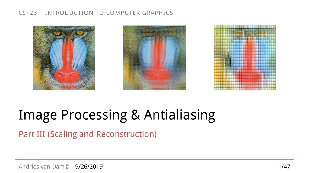
Image Processing & Antialiasing. Part III (Scaling and Reconstruction). Outline. Overview Example Applications Jaggies & Aliasing Sampling & Duals Convolution Filtering Scaling Reconstruction Scaling, continued Implementation.

E N D
Image Processing & Antialiasing Part III (Scaling and Reconstruction) 9/26/2019
Outline • Overview • Example Applications • Jaggies & Aliasing • Sampling & Duals • Convolution • Filtering • Scaling • Reconstruction • Scaling, continued • Implementation 9/26/2019
Image Scaling (assume no pre-filtering to remove the highest frequencies) Sample to get a discrete approximation of continuous signal (e.g., digital photo of real world) Reconstruct a continuous image definition (a more or less good approximation of original signal) Image scaling, rotation, … Resample signal to get pixel values for new discrete image, ready for raster display How/where should the signal be resampled? Different sampling methods depending on whether the image is scaled up or down 9/26/2019
Mapping: Samples, Reconstruction, and Filters • When we scale, we are trying to make a transformed version of the old discrete image • N new pixels will be derived from M old pixels. They probably won’t line up exactly. How to get new pixels? • Solution: Sample old image. Exactly where we sample is determined by size of old and new image • Example: Scaling image up from 10 x 10 pixels to 15 x 15 pixels • Need to generate 15 x 15 sample points; have 10 x 10 pixels • Given 15 x 15 samples across 10 x 10 pixels, must sample “in between” some pixels in old image: 10/15 = 2/3 units apart 9/26/2019
Sampling (during scaling-up) • Each pixel in new image will correspond to a sample point in old image • If sample point lies exactly on pixel in old image, then we could use that pixel value (using radius = 1 for optimal support width of optimal filter) • But what if our sample point lies somewhere between two old pixels? • If we could magically reconstruct “original” continuous picture represented by our 10 x 10 image, then we could resample it 15 x 15 times instead (like taking another picture) • Since we only have a discrete version we’ll take our best guess at what the original picture would have looked like • Using the old data, we will try to reconstruct the value at any arbitrary sample point on, or in between, our 10 x 10 pixels 9/26/2019
Resampling Reconstructed Image (1/3) • Resampling original image between integer pixel locations: best guess Each integer pixel location in the new transformed image corresponds to a real-valued sample location in the old image (not necessarily on pixel boundaries! In this case we must sample 15 times in a 10 pixel area, i.e., every 10/15 or 2/3 pixel intervals) Old Image: 10 Pixels New Image: 15 Pixels Good guesses Scaled intensity function with best guess on resulting inter-pixel sample values No guess needed SWAG: “simple wild-ass guess” 9/26/2019
Resampling Reconstructed Image (2/3) • Can think of image resampling as two distinct steps: • Reconstruct “original” continuous picture information from our discrete samples; although probably not correct, it’s the best we can do. Here we reconstruct with linear interpolation (triangle filter, S34) • Then, resample continuous data at mapped locations 9/26/2019
Resampling Reconstructed Image (3/3) • Display sampled values at their proper pixel locations in the transformed image. We have now scaled the image! Old image: 10 Pixels New image: 15 Pixels 9/26/2019
In-Class Question 1 9/26/2019
Discrete Reconstruction Why build this… …when you only need this? As shown later, we can do reconstruction and resampling stages in one step “Original” function is reconstructed ONLY at sample points needed for our new image. Why reconstruct entire continuous “original” image if we only need to sample at a few locations? Stay tuned… 9/26/2019
Outline • Images & Hardware • Example Applications • Jaggies & Aliasing • Sampling & Duals • Convolution • Filtering • Scaling • Reconstruction • Scaling, continued • Implementation 9/26/2019
Reconstruction Filters (1/2) • How to perform reconstruction to get (approximated) continuous image from sampled signal? • Use same filters from pre-filtering for removing high frequencies from continuous signals • Take as input a point where we want to sample the old image (can lie on or between pixels) • Guess the point’s value using weighted average of old image’s nearby pixel values (i.e., place filter at the point and do discrete convolution there) • Discrete convolution is much easier than integrating over continuous differential areas (which we don’t have anyhow, since we start with a pixel array) 9/26/2019
Reconstruction Filters (2/2) • In general, the better a filter estimates the original signal, the more expensive • We want to find a good middle ground between cost and quality • Review of general traits of filters: • Take weighted sum of pixel values near sampled point • Pixels further away are less influential; max weight at center of filter • Area covered by filter—called support—is centered around sample point and while infinite in extent for sinc, clearly is finite in discrete case) • Normalize area under filter to sum to 1 • Ensures transformed image will have same overall brightness as original image • Play with different filter shapes using scaling applet (shown in last lecture) • https://cs.brown.edu/courses/cs123/demos/scaling/index.html • Problem: to get discrete image in the first place prior to reconstruction/scaling, we scanned it in – is that pure point-sampling, f(x) f(k)? 9/26/2019
Scanning as Unweighted Area Sampling (Box Filter) (1/2) • In an idealized image processing pipeline, sample original continuous image to store as a pixel array, and then reconstruct a new continuous image using a filter. Resample it and scale to get new, scaled image • Look at scanning a photo using CCD (Charge-coupled device) scanner or taking a digital camera image, to understand sampling/reconstruction in spatial and frequency domains • CCD is a collection of light sensors that convert photons into electrons. Each light sensor on the CCD produces an electrical charge corresponding to the amount of light falling on it (Hertz 1887, Einstein 1905 re photoelectric effect) • Scanning “continuous” photograph or taking a digital picture results in unweighted area sampling: each rectangular element responds to total amount of light falling on it, without regard for how the light is distributed across the sensor! • This constitutes pre-filtering (before sampling and reconstruction!) with a box filter – introduces corruption because box filtering is multiplication with sinc in frequency domain! • NOT ideal low-pass filtering to cut out unrepresentable high frequencies (Nyquist)! Scanner CCD array (1 dimensional) Camera CCD array (2 dimensional) 9/26/2019
Scanning as Unweighted Area Sampling (Box Filter) (2/2) • Look conceptually at the process of scanning a continuous image/3D world using theoretical model of pre-filtering each scan line’s f(x), followed by sampling • Pre-filtering (with bad box filter): • Scanner does box filtering (unweighted area sampling) in spatial domain (CCD’s fault; not continuous, not ideal filter) • Dual is sinc multiplication in the frequency domain • Produces intermediary continuous signal f’(x): mostly band-limited to maintain frequencies near zero but has corrupting negative lobes, has rapid fall-off from center instead of 1, and doesn’t completely eliminate high frequencies • Sampling: • Sample f’(x); yield discrete pixels Pi,(information we store about image) • Intensity of Pidetermined by signal from ithCCD element • Thus sample Pirepresents corrupted version of original intensity of that area; cannot represent original exactly, but it is best we can (and it does beat point sampling!) 9/26/2019
Revisit Sampling • To understand reconstruction, we need to look at sampling from a mathematical point of view • You no doubt expect that evaluating any function f at evenly spaced points along the domain is just simple sampling… • Actually, we must do something that will seem unintuitive at first but will make sense by the end • Remember the goal of sampling is to represent the function as faithfully as possible… 9/26/2019
Sampling any f(x) with a Unit Comb • First thought: multiply scanline signal by a sampling function that is zero everywhere and 1 only at (integer) sample points, i.e., a unit “comb” • But to understand the ramification of multiplying with the unit comb in the spatial domain, we must compute its dual (to convolve it with dual of signal) • Determining a dual is computing the Fourier transform (see Section 18.11), and the resulting integration of the unit comb would equal 0, i.e., no frequencies! Spatial domain Frequency domain 1 9/26/2019
Sampling f(x) with a Dirac Delta (δ) Comb (1/2) • Instead the math dictates we use a comb of Dirac δs (aka impulses) - each δ has arbitrarily large value at its sample point but unit area - mathematical artifice • The dual of a comb of Dirac δsis another comb of Dirac δs • Sampling by multiplying f(x) by a Dirac δ comb in the spatial domain corresponds to convolving the dual of f(x) with the dual of the comb in the frequency domain (IP-II S59) (N.B.: we aren’t actually going to sample by multiplying with a δ comb) • The higher the sampling frequency, the better for reconstruction, and the more the δs in the frequency domain comb will be spread out (soon you’ll see why that is good!) Spatial domain Frequency domain 9/26/2019
Sampling f(x) with a Dirac Delta (δ) Comb (2/2) • Making sense of this: • The claims of the previous slide are almost all false… • They’re also almost true… • The truth involves limits • We're going to show you a little bit of how that works • Start not with infinitely thin, infinitely tall boxes (δ’s), but with wider boxes of finite height... 9/26/2019
Sampling with Step Functions • Multiplying an arbitrary continuous function with a unit step (1x1) and taking the area under that curve produces the average of that curve in that interval • Think of a unit-wide block of ice cut from a wavy sea melting in a bucket of unit width • Shrink the width to ½ but scale the height of the function by 2, and you’ll get an average of the function over a smaller interval • In the limit, you’ll take the area under a product which is very, very tall but has near-zero width and will approximate the actual value of the function at the sample point, the average over an infinitesimal segment of the function • The actual shape of the sampling function doesn’t really matter – it is an area argument • You can think of this as just "evaluate the function at the point" 9/26/2019
Revisit the Dirac Delta δ - not a true function • Think of it as a limit in a sequence of narrowing, ever taller, Gaussians (or rectangles) – a very tall and thin spike with unit area • If you successively multiply some signal f by each Gaussian in the sequence • get a mostly-small product, except near x = 0 • near 0, you get an increasingly large multiple of f(0) • …fading off in an increasingly narrow interval • areas under resulting product curves approach f(0) (see previous slide) • So “multiplying by δ and integrating” (i.e., convolving) at 0 gives f(0) • True for any x, get f(x) - therefore, convolving with δ gives back f – it’s the “identity” for convolution • If f discontinuous at 0, subtle things happen, e.g. get the average of the two values of a step function – see Section 18.8 • Real-world signals are effectively never discontinuous – our eye has to integrate photons over time, true essentially for all measurements 9/26/2019
δComb in Spatial Domain -> δComb in Frequency Domain Spatial domain Frequency domain • A δ comb in the spatial domain maps to another δ comb in the frequency domain • Easiest way to see this is to look at increasingly “δ comb-like” functions in both the spatial and frequency domain • Notice how as the function adds more “teeth”, the frequency spectrum widens to reflect this • Taken to the limit (imagine letting each δ tooth of the comb get thinner while more teeth are added) we get the δ comb to δ comb mapping • Math note: the fall-off allows this step function to have a Fourier Transform 9/26/2019
Sampling Introduces Infinite Replicas of a Spectrum • Sampling (evaluating f(x) at discrete values) corresponds to multiplication (in the spatial domain) of the original signal by a δcomb function (infinite sequence of impulses at the sample points) • Fourier analysis says that an impulse comb in the spatial domain transforms into another impulse comb in the frequency domain (S21) • Squeezing to increase sampling frequency in the spatial domain maps to stretching in the frequency domain • Multiplication in the spatial domain maps to convolution in the frequency domain • Convolving with an impulse comb replicates the function at every “tooth” of the comb – recall that convolving at 0 replicates the function, ditto for any x • Summary: when we sample by multiplying the spatial function by an impulse comb function, we convolve its frequency dual with another dual impulse comb, which leads to infinitely repeating frequencies 9/26/2019
Sampling with a Dirac Impulse Comb Replicates Spectrum Original Function (dual in frequency domain) Comb function (dual in frequency domain) * = Sampled Function (frequency domain) 9/26/2019 And if sampling frequency is too low, the spectra overlap and corrupt!
In-Class Question 2 Spatial domain 9/26/2019
Review • Mathematically, sampling = multiplication by δ comb in spatial domain • We’ll see that we don’t do this in practice, just do finite convolution with filter function • Look at the consequences in the frequency domain • There, it is convolution with δ comb • Produces infinite replicas of spectrum • For too low sampling rate replicas will overlap and thus will corrupt! • Therefore need band-pass filtering to eliminate replicated spectra and their arbitrarily high frequencies 9/26/2019
How Do We Kill All Replicas Due to Sampling? • We remove all but original band-limited spectrum ideally by multiplying with low-pass box filter in the frequency domain, which once again corresponds to convolving with sinc in the spatial domain Spatial to Frequency Frequency to Spatial 9/26/2019 Sinc filter
Reconstruction Filters to Kill Replicas • Practically, use cheaper filter such as truncated Gaussian or triangle to remove replicas in the frequency domain • Approximate reconstruction filtering with triangle in spatial domain: • Leaves higher frequencies • Will cause some aliasing, but comparatively insignificant • Later: pre-filtering to undo effects of box filtering and reconstruction filtering can be condensed to single filtering step • Remember: we do discrete convolution of samples with filter by placing filter at consecutive sample points (either at pixels or in between them, if image is scaled) and doing weighted averaging • Small filter size means relatively few pixels contribute 9/26/2019
Sampling and Reconstruction Filters: Sinc Adequate sampling rate, spectra are replicated but overlap little, minimizing corruption a) Original signal b) Sampled signal, replicated spectra c) Sampled signal ready to be reconstructed with sinc. d) Signal reconstructed with sinc (good approximation) 9/26/2019
Sampling and Reconstruction Filters: Triangle a) Original signal b) Sampled signal, replicated spectra e) Sampled signal ready to be reconstructed with triangle f) Signal reconstructed with triangle (not bad!) (Courtesy of George Wolberg, Columbia University.) 9/26/2019
Reconstruction Filters: Inadequate Sampling Rate: Sinc Inadequate sampling rate so spectra overlap and significant corruption/aliases (compare a and d) a) Original signal b) Sampled signal c) Sampled signal ready to be reconstructed with sinc d) Signal reconstructed with sinc (note aliasing!) 9/26/2019
Reconstruction Filters: Inadequate Sampling Rate: Triangle Inadequate sampling rate so spectra overlap and significant corruption/aliases (compare a and d) a) Original signal b) Sampled signal c) Sampled signal ready to be reconstructed with triangle d) Signal reconstructed with triangle (even worse!) sinc from previous slide 9/26/2019
In-Class Question 3 9/26/2019
Moral of the Story… Inadequate sampling rate defeats even the perfect box/sinc low pass filter because of overlapping spectra Now let’s again look at different filter shapes 9/26/2019
1/2 1/2 -1 < x < 1 x ) B ( elsewhere 0 Box Filter with 2 unit support (1/2) 1/2 -1 1 • We can create a 2 unit box filter B: • Graph representation of B: • Reconstructing with B as filter “draws bars”: • Box filter has discontinuities at boundaries, discrete convolution must be special cased: • At old pixel locations: just use pixel values • Everywhere else: use box filter (covers two pixels); value is just unweighted average of two neighboring pixels • Not bad for signals with large constant areas, sudden transition between differing values 9/26/2019
Box Filter with 2 unit support (2/2) • Lousy for steadily varying signals, for instance, sin(x) 9/26/2019
Triangle Filter (1/3) Triangle filter T: This normalized filter with 2 unit support approximates sinc filter of optimal width 2 Acts as linear interpolation filter. Takes weighted average of neighboring pixel values according to distance from sample point, i.e., “connect the dots” 9/26/2019
1.0 Filter value at x0 = 1.0Pixel value at x0 = 0.8Filterx0• Pixelx0 = 0.8 Triangle Filter (2/3) • If we center triangle filter directly over pixel in source image, it returns that pixel’s value: • What happens when we sample halfway between pixels in source image? • Intuition: would expect it to return average of two pixel values. Intuition is correct: Filter value at x0 = 0.5, Pixel value at x0 = 0.8 Filter value at x1 = 0.5, Pixel value at x1 = 0.5 Filterx0 • Pixelx0 = 0.4, Filterx1 • Pixelx1 = 0.25 Fx0 • Px0 + Fx1 • Px1 = 0.65 9/26/2019
Triangle Filter (3/3) • Similarly, if filter is 30% towards one pixel and 70% towards another, will return average of two pixels weighted by 30% and 70%; it linearly interpolates See the discrete convolution applet (seen in previous lecture): https://cs.brown.edu/courses/cs123/demos/convolutions/discrete-convolutions.html Weight = 0.3•P0+ 0.7•P1 9/26/2019
Avoiding Continuous Convolution • Whatever reconstruction filter we use, save work by combining reconstruction filtering with resampling the reconstructed signal • Re-sample at a discrete number of points determined by the image transformation, e.g., scaling • Do this by placing the reconstruction filter at sample points only and evaluating discrete convolution there • But what ARE those sample points for scaling? We saw scaling up involves sampling “in between” image pixels • Scaling down adds additional complexity, as we’ll soon see 9/26/2019
Scaling up by 2.0: source(x) dest(2x) Scaling: Forwards Mapping • In forward direction multiple pixels in source contribute to each pixel in destination, and each pixel in source contributes to multiple pixels in destination • Determining which destination pixel a group of a source pixels contribute is not the best method • Example: Scaling up by 2 • Pixel “1” in source contributes to pixels “1,” “2,” and “3” in destination • Pixel “3” in destination is contributed to by both pixels “1” and “2” in source 9/26/2019
Source Image Sample points Instead, we back-map this way: We don’t forward map this way: dest(x) source(x/a) source(x) dest(a*x) Scaling: Backwards Mapping • Where to place filter in source image? • Compute sample points by back-mapping from destination back to source image • Backwards map • For each pixel in destination, which pixels in source contribute to it? • Determined by placing filter in source image as function of scale factor • Backwards mapping is inverse of the image transformation, e.g., if we scale source up by 2.0, then map each pixel x in destination from pixel x/2 in source image For each pixel, x, in destination image, sample x/2 from source image Scaling up by factor a: 9/26/2019
In-Class Question 4 9/26/2019
Timeout – review of some fundamental concepts (1/4) • We can characterize signals either in their original domain or by their component frequencies and amplitude – thus we get the notion of dual domains (spatial and frequency) and dual operations (convolution and multiplication) • The simplest wave form is a periodic sine • Ignore the mathematically induced negative part of the spectrum, and the term at the origin: this "DC" (for direct current, as opposed to AC, alternating current) term is the average energy in the signal - real spatial or acoustic energy has sine waves not centered at y=0 but y=c. • Can decompose more complex wave forms (both periodic and aperiodic) in a (infinite) sum of sines and cosines (Fourier analysis/synthesis) Signal Domain DC Frequency Domain 9/26/2019
Timeout – review of some fundamental concepts (2/4) • Frequency spectrum plots amplitude at each frequency, typically a fundamental and its harmonics in the acoustic domain • These frequencies and their amplitudes are determined by Fourier Analysis, a process too complex to explain in this course • It suffices to know that a signal can be decomposed into a sum of sines and cosines • A sine in the spatial or signal domain is represented by a single frequency in the frequency spectrum, and each sine in the sum will be represented by one amplitude at that frequency • These signals are all in the spatial domain and we do not show the frequency domain here • Note that image wave forms don’t show periodicity typically even though they can be decomposed into periodic functions! 9/26/2019
Timeout – review of some fundamental concepts (3/4) • In general, rapid fall-off of amplitude with higher frequencies, so filtering them out doesn't lose vital information from the signal • Leaving them in would cause aliases that corrupt the reconstructed waveform Multiplied by perfect box filter in the frequency domain (convolution with sinc in the spatial domain) 9/26/2019
Timeout – review of some fundamental concepts (4/4) • We look at signals as intensity functions (waveforms) of space (images) or time (acoustic) • Filters similarly are 2D, but for images, the filters are actually 3 dimensional (e.g., triangle becomes circular cone or rectangular pyramid, Gaussian has its 3D shape, etc.) W 9/26/2019 Circular cone and Gaussian filter Pyramid filter Sinc filter