Download
1 / 16
160 likes | 287 Vues
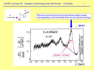
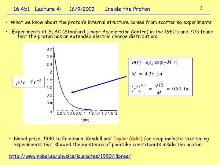
1. 16.451 Lecture 4 : 16/9/2003 Inside the Proton. What we know about the proton’s internal structure comes from scattering experiments Experiments at SLAC (Stanford Linear Accelerator Centre) in the 1960’s and 70’s found

E N D
1 16.451 Lecture 4: 16/9/2003 Inside the Proton • What we know about the proton’s internal structure comes from scattering experiments • Experiments at SLAC (Stanford Linear Accelerator Centre) in the 1960’s and 70’s found • that the proton has an extended electric charge distribution: • Nobel prize, 1990 to Friedman, Kendall and Taylor (Cdn!) for deep inelastic scattering • experiments that showed the existence of pointlike constituents inside the proton: • http://www.nobel.se/physics/laureates/1990/illpres/
detector Before After proton “Form factor” gives Fourier transform of extended charge distribution 2 Overview: Electron scattering experiments: (Ref: Krane 3.1) electron scatters from the proton’s electric charge distribution (r) Scattering rate is determined by the cross-section: point charge result (known)
3 What it looks like: proton electric form factor 4 – momentum transfer: Q2 Ref: Arnold et al., Phys. Rev. Lett. 57, 174 (1986) “Dipole formula” (Inverse Fourier transform gives charge density (r))
4 Details, Part I: Scattering Cross Section: , d/d scattered particle beam target • A beam particle will scatter from the target at any angle if it approaches within a • (perpendicular) cross sectional area centered on the target particle. • Definition:total scattering cross section (units: area, eg. fm2) • Scattering into a particular solid angle at (,) in 3d occurs if the beam particle • approaches within a (perpendicular) cross sectional area d/d centered on the target • Definition:differential scattering cross section d/d (units: area/solid angle)
Cross-sectional area: proton, R ~ 0.8 fm 5 Units, etc: What is the right scale for ? WRONG! Geometry has nothing to do with the value of . Scale is set by the interaction and beam energy Cross section unit: “barn” 1 barn = 10-24 cm2 = 100 fm2 : b d/d: b/sr Scale for proton-proton scattering: ~ 0.01 b Other reactions: -p: ~ 10-14 b e-p: < 10-9 b but energy-scale dependent!
beam Interaction probability: Transmission:T(x) = probability of getting to x without interacting = 1 – P(x) T(x+dx) = T(x) [1 – dP] = T(x) [1 – nt dx] beam 6 Connection to Experiment: • Experimenters measure the scattering rate into a given solid angle at (, ). • Knowing target thickness, detector efficiency and solid angle yields d/d nt = # of target nuclei per unit volume
7 Targets: thick and thin! A target is said to be “thin” if the transmission probability is close to 1. Then, for target thickness x: thin target: Otherwise, attenuation in the target has to be accounted for explicitly via the exponential relationship: (always correct) Thick target: P(x) 1, essentially independent of x beyond a certain thickness.
8 connection to experiment continued.... target, L detector efficiency rate I() scattered P() beam rate Io (thin target case!)
9 Electron scattering apparatus at SLAC: magnetic spectrometer target shielded detector package beam
10 Details, Part II: Statistical Accuracy in Experiments (Krane, sec. 7.5) Suppose we perform a scattering experiment for a certain time T. The differential cross section is determined from the ratio of scattered to incident beam particles in the same time period: Scattering is a statistical, random process. Each beam particle will either scatter at angle or not, with probability P(). Individual scattering events are uncorrelated. In this case, the statistical uncertainty in N() is said to follow “counting statistics”, and the error in N() determines the statistical uncertainty in d/d: (Note: strictly speaking, N >> 1 for the Gaussian distribution to apply, but this is the usual case in a scattering experiment anyway.)
11 Interpretation of “counting statistics” error: If we perform the same experiment many times, always counting for the same time T, we will measure many different values of N, the number of scattered particles... the distribution of values of N, call this Ni, will be a Gaussian or Normal distribution, with the probability of observing a particular value given by: with standard deviation: and mean value: If we only do the measurement once, the best estimate of the statistical error comes from assuming that the distribution of events follows counting statistics as above. However, it is important to verify that this is the case! (Electrical noise, faulty equipment, computer errors etc. can lead to distributions of detected particles that do not follow counting statistics but in fact have much worse behavior. This will never do! ..... )
solid line: fitted Gaussian function Sum of entries = total number of measurements, M Mean value: A = - ( 0.9 0.9 ) x 10-5 -- very good agreement with counting statistics based on values of N+ and N- 12 Example: checking on “counting statistics” “Gamma Ray Asymmetry” histogram, Ph.D. thesis data (SAP)
13 continued... • Notes: • Time T required to achieve a given statistical accuracy: • Beam time is expensive, so nobody can afford to waste it! • e.g. at Jefferson Lab: 34 weeks/year x 2 beams costs US$70M (lab budget) • $625k Cdn/hour! • 3. Efficient experiment design has statistical and systematic errors comparable, • counting rate optimized for “worst” data point (d/d smallest) • see example, next slide...
14 Data from High Energy Electron-Proton Scattering at SLAC: Note log scale! cross section drop like 1/Q4 – most of the time is spent at the highest Q2 data point! Q2= 31 GeV2, N = 39 counts / = 8% Q2= 12 GeV2, N = 1779 counts / = 2% Ref: Sill et al., Phys. Rev. D 48, 29 (1993) (Statistical errors only shown)
15 Tables from Sill et al. SLAC experiment, 1993 Independent systematic errors added in quadrature to the statistical error: Beam energy and spectrometer angle adjusted to vary the parameter of interest, momentum transfer Q2
16.451 Homework Assignment #1 Due: Thursday Sept. 25th 2003 Note:I will be traveling on Sept. 25 and leaving my office by 3 pm. Assignments handed in after that time will count as “late”, should be submitted to the department office for a date and time stamp, and will be collected Monday – SAP. 1.Penning trap problem:(Review your class notes from lectures 2 and 3.) Use the equations ofmotion for trapped particles to work out expressions for the (modified) cyclotron frequency c’, the axial frequency z and the magnetron frequency m .in terms of the fundamental particle and trap parameters. (Note: assume that m << c and work this one out first in order to simplify the task of evaluating c’.) For each type of motion, draw a sketch of the associated particle orbit and explain in simple terms how it comes about. Evaluate the three frequencies numerically for a proton in a Penning trap with magnetic field B = 6.0 T, electrode potential Vo = 100 V, and trap dimension d = 3 mm. What is the radius of the proton’s orbit if no axial motion is excited and the total energy is 100 ħ c ? 2. Hyperfine splitting in hydrogen: (Review lecture 3 and refer to Krane, sections 16.3-4.) Use a semiclassical Bohr model of the hydrogen atom to estimate the hyperfine splitting between the F = 0 and F = 1 total angular momentum states. (Assume that the energy splitting is due to the interaction between the magnetic moments of the proton and electron.) Draw a diagram to illustrate your approach to the calculation; verify that the energy splitting should be proportional to the dot product of electron and proton spin vectors, and compare your numerical value to the measured value for the hydrogen atom. 3. Counting Statistics: (Review class notes for lecture 4 and Krane, section 7.3) a) Look closely at the graph from lecture 4 showing the gamma ray distribution that was analyzed to test for counting statistics behavior and draw a hand sketch of what it looks like. Write down an expression for the Gaussian distribution function that would have been fitted to the data to obtain the solid curve. Use the scales in the graph, and this formula, to estimate the standard deviation of the distribution, and the number of measurements M; from these data, show that the stated error in the mean ( 0.9 x 10⁻⁵) is consistent with the distribution of measurements. b) (Krane, problem 7.13) A certain radioactive source gives 3861 counts in a 10 minute counting period. When the source is removed, the background alone gives 2648 counts in 30 minutes. Determine the net source counting rate (counts per second) and its uncertainty, explaining your reasoning. (Treat the measurements of “background” and “signal” events in a counting experiment as independent.)