Download
1 / 41
490 likes | 863 Vues
16. Theory of Ultrafast Spectroscopy or Feynman Diagrams Made Simple. Nonlinear-Spectroscopic Experiments: Limiting Cases. Medium to be studied. Frequency Domain. or. cw monochro- matic beams. Time Domain. delta-function pulses. or. where.

E N D
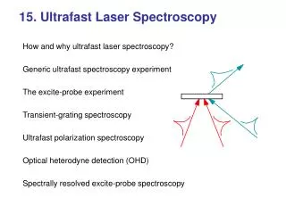
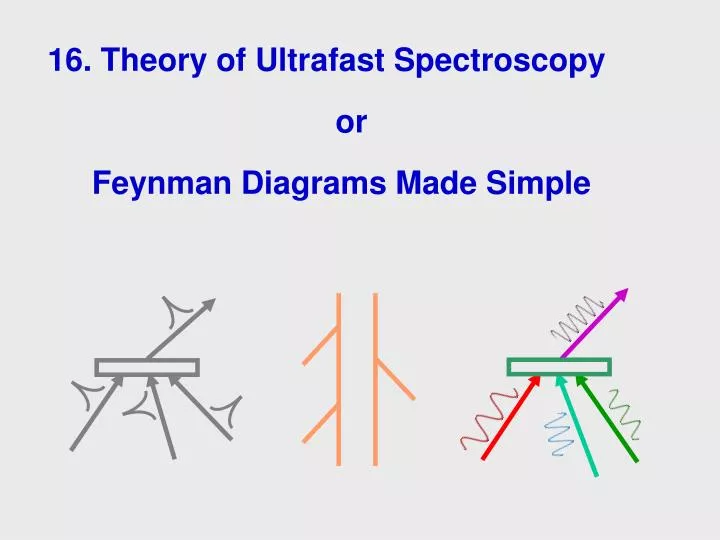
16. Theory of Ultrafast Spectroscopy or Feynman Diagrams Made Simple
Nonlinear-Spectroscopic Experiments:Limiting Cases Medium to be studied Frequency Domain or cw monochro- matic beams Time Domain delta-function pulses or where
Ultrashort laser pulses are an intermediate case. time Ultrashort laser pulses are really short, so they appear to be time-domain experiments waiting to happen. But, unlike true d-function pulses, they have finite bandwidth. So they can be resonant or nonresonant. This will be the key.
Ultrafast-Spectroscopy Experiments:An Intermediate Case b b Resonant time domain a Nonresonant frequency domain a b g a b a Ultrashort pulses have large, but finite, bandwidth. So experiments using them can be resonant or nonresonant. In addition, ultrashort-pulse experiments can be “nearly resonant.” This involves much more complex formulas. We won’t treat this case. Also, ultrashort-pulse experiments can be nonresonant for some input pulses and resonant for others. We can treat this case.
Feynman Diagrams Made Simple Quick quantum-mechanical derivation Nonlinear-optical Feynman diagrams in the frequency domain—cw experiments Example and tricks Nonlinear-optical Feynman diagrams in the time domain—delta-function-pulse experiments Example and tricks Feynman diagrams for experiments with simultaneous time- and frequency-domain character—ultrashort-pulse experiments The “ultrashort-pulse domain” Examples and tricks
A Sneak Preview of Feynman Diagrams Each diagram corresponds to a term in a complex sum. We use such diagrams because they’re easier to remember than the actual equation. A Feynman diagram can be interpreted in the time or frequency domains. Time domain Frequency domain d d g g w3 a, b, g, and d represent states. t3 b b t2 w2 w1 t1 a a a a delta-function pulse inputs at times, t1, t2, and t3 cw beam inputs of frequencies, In both domains, the particular ordering of the pulse times or beam frequencies is referred to as a time-ordering. Many time-orderings contribute to the total response/susceptibility.
Semiclassical Nonlinear-OpticalPerturbation Theory Treat the medium quantum-mechanically and the light classically. Assume negligible transfer of population due to the light. Assume that collisions are very frequent, but very weak: they yield exponential decay of any coherence Use the density matrix to describe the system. Effects that are not included in this approach: saturation, population of other states by spontaneous emission, photon statistics.
The density matrix b w a If the state of a single two-level atom is: ρaa(t) or ρbb(t)are the population densities of states a and b. The density matrix, rij(t), is defined as: When laser beams with different k-vectors excite the atom, rij(t) tends to have a spatially sinusoidal variation. A grating is said to exist if ρaa(t) or ρbb(t)is spatially sinusoidal, A coherence is said to exist if rab(t) or rba(t) is spatially sinusoidal.
The density matrix For a many-atom system, the density matrix, rij(t), is defined as: where the sums are over all atoms or molecules in the system. Simplifying: The diagonal elements (gratings) are always positive, while the off-diagonal elements (coherences) can be negative or even complex. So cancellations can occur in coherences.
Why do coherences decay? A coherence is the sum over all the atoms in the medium. The collisions "dephase" the emission, causing cancellation of the total emitted light, typically exponentially.
Grating and coherence decay: T1 and T2 A grating or coherence decays as excited states decay back to ground. A coherence can also cancel out if each atom has different phase. The time-scales for these decays to occur are: Grating [raa(t)or rbb(t)]: T1 “relaxation time” Coherence [rab(t) or rba(t)]: T2 “dephasing time” Collisions dephase; so, except in dilute gases, T2 << T1. The measurement of these times is the goal of much of nonlinear spectroscopy!
Nonlinear-Optical Perturbation Theory The Liouville equation for the density matrix is: (in the interaction picture) which can be formally integrated: which can be solved iteratively: Note that i.e., a “time ordering.”
Perturbation Theory (continued) Expand the commutators in the integrand: Consider, for example, n = 2: Thus, contains 2n terms.
Perturbation Theory (continued) Now, V is the perturbation potential energy due to the light and is of the form, , where E is the total light electric field. But V is in the interaction picture, so we have: where: [Note that U(t) U*(t’) = U(t-t’) ] So a typical term looks like: is also in the interaction picture: Dividing out these U(t)’s yields: Notice that time propagates from to to t along two different paths.
Perturbation Theory (continued) So a typical term (in second order) is: But, in nth order, the E-field is typically the sum of n input light fields: As a result, each of the above type of terms expands into many terms. Allowing each field to occur only once yields n! as many more. Thus, in nth order, there are 2nn! terms!
How do we remember all these terms? Use diagrams! Consider two input beams and this second-order term, noting that time propagates from t0 to t along two paths: time
Perturbation Theory (cont’d) w1 w2 Now expand in terms of the atomic eigenstates: For our second-order term, for example: we find: Computation of the number of terms now is an exercise left to the student…
Doing the integrals… [ Set t0 = 0 ] Dipole moment matrix elements at the ith beam polarization Now, to go further, we’ll consider limiting cases.
Including dephasing w1 w2 Before we evaluate these integrals, we must include dephasing. Every time a transition frequency occurs, we must subtract off the dephasing rate for that transition. This is the usual method for adding width to a transition. Thus: This addition comes from a complex analysis that takes into account collisions. Now we can do the integrals in the various cases.
The Frequency Domain w1 w2 Evaluating a single second-order term for monochromatic fields yields: where and where: The (-1) occurs in terms with an odd number of V(t)’s to the right of The factor of is the population density of the initial state. The factors of are dipole-moment matrix elements between the states a and b for the polarization of beam k. The denominators contain the line shape--the dynamical information.
Drawing Feynman Diagrams in the cw Limit • Draw two vertical line segments. • 2. Draw a rightward-pointing diagonal arrow for each input field. Upward-pointing arrows correspond to absorbed photons, and downward-pointing photons correspond to emitted photons. Choose an ordering for these “interactions,” and also choose which side each should appear on. Label each interaction with a light frequency. • 3. Write in states (a, b, c, d, e) at the base and just above each interaction. Every possible diagram of this form corresponds to a term in the expression for c(n), where n is the number of interactions. This diagram corresponds to:
Drawing Feynman Diagrams in the cw Limit Include a factor of –1 if there are an odd number of interactions on the right: Diagram Include a factor of the initial population density of the state at the base of the diagram:
Drawing Feynman Diagrams in the cw Limit Piece of diagram At each interaction, we write down a dipole-moment matrix element: “(1)” means “for the polarization of beam 1” After each interaction (reading upward), we write a resonant denominator of the form: Diagram where
Interpreting Feynman Diagrams in the cw Limit The contribution to c(n) is the product of all factors shown below: Resonant denominator: Resonant denominator: Resonant denominator: Resonant denominator: Matrix elements: The population density of the state at the base: Two interactions on the right (a factor of –1 for each): (-1)2
Example: Linear Optics—The Absorption Coefficient and Refractive Index vs. Frequency Linear optical problems involve only one photon: Resonance frequency Dephasing time Light frequency This is just the well-known complex Lorentzian line shape, whose even (imaginary) component is the absorption coefficient and whose odd (real) component is the refractive index.
How do you know which diagrams to include? w1 w2 First consider the process, and include only the most resonant, and hence strongest, terms. For example, consider difference-frequency generation, Maximally resonant denominators: Anti-resonant denominators:
Example: Higher-Order Wave Mixing 12-wave mixing Signal frequency:
A 12-Wave-Mixing Feynman Diagram All denomi-nators are maximally resonant. Unfortunately, there are about 10,000 more such diagrams to consider…
Drawing Feynman Diagrams in the Time Domain time t4 t3 t2 t1 Now, suppose that the input light is a sum of delta-function pulses. The relevant variables are now the pulse relative delays, t t1 t2 We can now write Feynman diagrams for this class of processes, but we must label the interactions with times, rather than frequencies. Every possible diagram of this form corresponds to a term in the expression for the response, R(n), where n is the number of interactions.
The Time Domain: d-function pulses The integrals are now even easier. Note that the result is a product of propagators.
Interpreting Time-Domain Feynman diagrams t4 t3 t2 t1 As before, include a factor of –1 if there are an odd number of interactions on the right: As before, include a factor of the initial population density of the state at the base of the diagram. Also, as before, at each interaction, we write down a dipole-moment matrix element: Instead of resonant denominators, we write simple exponential propagators:
Example: The Linear Response As before, linear optical problems involve only one photon and use the same diagram: where . Dropping the subscript, 1: Resonance frequency Dephasing time This is just the well-known fact that the molecules oscillate at their own frequency, emitting “free-induction decay,” and dephase exponentially. The Fourier transform of this response is the complex Lorentzian line shape, whose even component is the absorption coefficient and whose odd component is the refractive index.
Example: The Excite-Probe Experiment Coherence spike Excited- State decay Photon echo (PFID) Delay, Excitation pulse Observe change in probe- pulse energy vs. delay, Probe pulse The observed signal vs. delay is complex, with three components:
The Excite-Probe Experiment (cont’d) Signal pulse The excite-probe experiment is a third-order process, with the excitation pulse providing two photons: Probe pulse Excite Pulse(s) Only state a is populated initially. Coherence spike Photon echo (PFID) Excited- state decay Delay,
The intermediate domain: ultrashort pulses Ultrashort pulses have finite bandwidth and finite pulse length. Can we define Feynman diagrams for nonlinear-optical experiments with them? Yes! All the integrals are of the form: For ultrashort pulses, two important cases yield simple results. Case 1. Resonant excitation: Set E(t) = time domain Case 2. Nonresonant excitation: Set E(t) = constant frequency domain
The Ultrashort Pulse Domain (cont’d) Purely resonant ultrashort-pulse experiments are pure time-domain experiments, and we use the time-domain Feynman diagrams. Purely nonresonant ultrashort-pulse experiments are pure frequency- domain experiments, and we use the frequency-domain Feynman diagrams. What about experiments that are resonant at some steps and nonresonant at others? Resonant steps, so label with times Nonresonant steps, So label with frequencies
But can we define rules for interpreting this “time-frequency” hybrid diagram that make sense? Yes! Doing the integrals, we see that time-domain steps yield the same factors, But frequency-domain (nonresonant) steps yield slightly different denominators (we must take into account the existing coherence from the previous time-domain step). Also any resonant pulse must be simultaneous with all nonresonant pulses prior to it since the last resonant step. Here, for example, pulses 1 and 2 must be coincident in time (same for 3 and 4). Propagator: Resonant denominator: Propagator: Resonant denominator: Matrix elements: The population density of the state at the base:
Example: Femtosecond CARS 1 2 3 0 In fsec transient CARS, a two-photon Raman resonance is excited, and its decay is probed vs. delay, all by pulses. The decay of the coherence, wga, is to be measured by varying a delay. Propagator: Propagator: Resonant denominator: Signal Plotting the signal intensity vs. yields the dephasing time, T2ag:
Conclusions Nonlinear-optical Feynman diagrams better allow us to remember the large number of terms in the complex perturbation-theory expansion. We can define Feynman diagrams for several cases: general input fields cw input fields (frequency domain) delta-function input fields (time domain) ultrashort-pulse input fields: time or frequency-domain or both An understanding of nonlinear-optical Feynman diagrams can make almost any nonlinear-optical or nonlinear- spectroscopic problem (and even linear ones!) relatively easy!